Network meta-analysis of multi-environment trials with linear mixed models in ASReml-R
Meta-analysis combines treatment effects across studies to produce a single, more precise summary. The classical version extracts one effect size per study (a difference in means, a log odds ratio, a standardized response) and pools those values. That logic works cleanly for two treatments, but agricultural and biomedical programs rarely test the same two treatments everywhere. They test overlapping subsets: trial A compares treatments 1 and 2, trial B compares 2 and 3, and no single trial contains all treatments at once.
Network meta-analysis (NMA), also called multiple-treatments meta-analysis, is built for exactly this situation. It estimates and ranks several treatments simultaneously, including pairs that were never compared head to head. It does so by combining direct evidence (comparisons made within a trial) with indirect evidence (comparisons inferred through a shared treatment). If trial A gives 1 versus 2 and trial B gives 2 versus 3, the network supplies an estimate of 1 versus 3 through the common treatment 2.
This structure is the norm in multi-environment trials, where each site evaluates only a subset of treatments and the resulting study-by-treatment table is sparse and unbalanced. Pairwise meta-analysis handles such data poorly: it discards indirect evidence, analyzes each contrast in isolation, and ignores correlations among treatments within a study. A linear mixed model fitted to the whole network avoids all three problems. It recovers indirect evidence, models the correlation structure explicitly, and shrinks unstable study-level estimates toward the network mean, which stabilizes inference when data are thin.
This post focuses on summary-level NMA, where each treatment in each trial is represented by a mean and an associated sampling variance. This is the information typically reported in published field trials, particularly in plant pathology. A future post will treat individual plot-level data, which additionally supports spatial models, trial-specific error structures, and plot-level covariates.
The models below are fitted with ASReml-R, a commercial mixed-model package that excels at flexible variance-covariance structures. That flexibility is what makes the progression from simple to structured covariance models possible within a single, consistent framework.
Linear mixed models in one paragraph
A linear mixed model splits the systematic part of the data into fixed effects, whose individual values we want to estimate (here, treatment means and contrasts), and random effects, which we treat as draws from a distribution and summarize through variance components (here, the study-to-study variability of treatment performance). Fixed-effect estimates are BLUEs (best linear unbiased estimators); random-effect quantities are BLUPs (best linear unbiased predictors). BLUPs are shrunken toward zero by an amount that depends on how much information each study contributes, which is precisely the borrowing of strength that makes NMA work on sparse networks. Variance components are estimated by restricted maximum likelihood (REML), which corrects the downward bias that ordinary maximum likelihood (ML) introduces when fixed effects are estimated alongside the variances. Everything that follows is a specific choice of which effects are fixed, which are random, and what covariance structure the random effects carry.
Notation and the second-stage model
We follow the notation of Madden, Piepho, and Paul (2016), referred to below as the original manuscript, and we adopt their model labels (F1, F2, R1 through R5). Let \(y_{ij}\) denote the summary result (here, the mean yield) for study \(i = 1, \dots, K\) and treatment \(j = 1, \dots, m\). Each summary comes from a completed first-stage analysis and carries an estimated sampling variance \(s_{ij}^2\). The general model is
\[ y_{ij} = \eta_{ij} + e_{ij}, \qquad e_{ij} \sim N\!\left(0,\ s_{ij}^2\right), \]
where \(\eta_{ij}\) is the linear predictor for study \(i\) and treatment \(j\), and \(e_{ij}\) is the residual, that is, the estimation error inherited from the first stage. Collecting the treatments of study \(i\) into vectors \(\mathbf{y}_i\), \(\boldsymbol{\eta}_i\), and \(\mathbf{e}_i\), the model in matrix form is
\[ \mathbf{y}_i = \boldsymbol{\eta}_i + \mathbf{e}_i, \qquad \mathbf{e}_i \sim N\!\left(\mathbf{0},\ \mathbf{R}_i\right), \]
with \(\mathbf{R}_i = \operatorname{diag}(s_{i1}^2, \dots, s_{im}^2)\). The defining feature of a second-stage analysis is that \(\mathbf{R}_i\) is known, not estimated: the within-study uncertainty was already quantified in the first stage (there are alternatives to this that are not discussed here). We assume the treatment means within a study are conditionally independent given the study, which is justified for randomized complete block designs when \(s_{ij}^2\) is taken as one half of the squared standard error of a difference (see the original manuscript and references therein).
The models differ only in how the linear predictor \(\eta_{ij}\) is structured and in which variance-covariance matrix governs the between-study random effects. Two matrices recur:
- \(\boldsymbol{\Omega} = \operatorname{var}(\mathbf{u}_i)\), the between-study covariance of the random treatment-by-study deviations \(\mathbf{u}_i\), used when the study main effect is fixed.
- \(\mathbf{G} = \operatorname{var}(\mathbf{h}_i)\), where \(h_{ij} = \beta_i + u_{ij}\) combines the random study main effect \(\beta_i\) and the interaction \(u_{ij}\) into a single random vector \(\mathbf{h}_i\), used when the study main effect is random.
Loading packages
We load the working packages and import the wheat fungicide data from the original manuscript, which in turn derive from Paul et al. (2010). That study analyzed wheat yield across 136 field trials conducted over 12 years in 14 U.S. states. Each trial used a randomized complete block design and included at least a no-fungicide control and tebuconazole (Folicur). Other fungicides appeared in varying combinations, with four treatments per trial on average. The authors provide treatment mean yields and their sampling variances, the standard inputs for a second-stage analysis. The first-stage ANOVA has already been performed, so these summaries are the data for the network meta-analysis below.
The dataset contains:
trial: study identifiertrt: treatment code (10 = control, 2 to 6 = fungicides)yield: mean yield per treatment in each study (the summary effect size, \(y_{ij}\))varyld: within-study sampling variance of the mean (\(s_{ij}^2\), equal to1/wtyld)wtyld: inverse-variance weight (\(1/s_{ij}^2\), used in fitting)cla: wheat marketing class (S = soft, W = white), a potential moderatorgroup: study classification based on treatment combinations (13 groups)
pacman::p_load(
  here,       # find file
  janitor,    # clean column names
  tidyverse,  # data wrangling and visualization
  asreml      # mixed models via REML
)
## Online License checked out Fri Jun 5 10:18:21 2026Importing and preparing the data
We import the trial data, standardize the column names, recode the treatment labels, and convert yield from bushels per acre to metric tons per hectare. Because yield is rescaled by a constant \(c = 0.0628\), the sampling variance must be rescaled by \(c^2\) so that the weights stay on the correct scale. The weight is the inverse of the rescaled sampling variance.
dat <- read_csv(here("content", "project", "network meta asreml", "madden_2016.csv"), show_col_types = FALSE) %>%
  janitor::clean_names() %>%
  mutate(across(c(trial, trt, cla, group), as_factor)) %>%
  mutate(
    trt = fct_recode(trt,
      "Teb"    = "2",   # tebuconazole (Folicur)
      "Prop"   = "3",   # propiconazole (Tilt)
      "Prothi" = "4",   # prothioconazole (Proline)
      "ProTe"  = "5",   # prothioconazole + tebuconazole (Prosaro)
      "Metc"   = "6",   # metconazole (Caramba)
      "Chk"    = "10"   # no-fungicide control
    ),
    yield  = yield * 0.0628,            # bu/acre -> t/ha (scale by c)
    varyld = varyld * (0.0628^2),       # variance scales by c^2
    wtyld  = 1 / varyld                 # inverse-variance weight
  )

trt_levels <- levels(dat$trt)
n_trt <- length(trt_levels)
The six treatments are the control (Chk) and five fungicides: tebuconazole (Teb), propiconazole (Prop), prothioconazole (Prothi), prothioconazole plus tebuconazole (ProTe), and metconazole (Metc).
Fitting weighted second-stage models in ASReml-R
Every model below shares the same machinery for the known within-study variance \(\mathbf{R}_i\). Two arguments work together:
weights = "wtyld"tells ASReml-R that observation \(ij\) has weight \(w_{ij} = 1/s_{ij}^2\).family = asr_gaussian(dispersion = 1)fixes the residual scale parameter at 1 rather than estimating it.
Together these set the residual variance of \(y_{ij}\) to \(1/w_{ij} = s_{ij}^2\), which is exactly \(\mathbf{R}_i = \operatorname{diag}(s_{ij}^2)\). This is the central trick of summary-level meta-analysis: the first-stage uncertainties enter as fixed, known quantities, and REML is left to estimate only the between-study variance components. Forgetting to fix the dispersion would let the model rescale the supplied weights, which would no longer reproduce a meta-analysis.
ASReml-R fits all models by REML. The original manuscript gives the full model derivations and the corresponding SAS code; we reproduce a representative subset here and concentrate on the link between each formula, its covariance structure, and its R implementation.
Model F1: fixed study and treatment effects, homogeneous between-study variance
This is Equation 5 of the original manuscript. Both treatment and study are fixed, and a random treatment-by-study interaction absorbs the between-study variability of treatment performance:
\[ y_{ij} = \theta + \beta_i + \tau_j + u_{ij} + e_{ij}, \qquad u_{ij} \sim N\!\left(0,\ \sigma_u^2\right). \]
Here \(\theta\) is the intercept, \(\beta_i\) the fixed study main effect, \(\tau_j\) the fixed treatment main effect, and \(u_{ij}\) the random study-by-treatment deviation. “Homogeneous” means a single \(\sigma_u^2\) for all treatments, so the between-study covariance matrix is \(\boldsymbol{\Omega} = \sigma_u^2 \mathbf{I}_m\), with no covariance among treatments. Because study is fixed, treatment contrasts are estimated from intrastudy information only: each \(\tau_j - \tau_{j'}\) rests on comparisons made within the same trial, which respects the principle of concurrent control.
mod.f1 <- asreml(
  fixed  = yield ~ trt + trial,                 # fixed treatment and study
  random = ~ trial:trt,                          # random study-by-treatment, single variance
  weights = "wtyld",                             # w_ij = 1 / s_ij^2
  data    = dat,
  family  = asr_gaussian(dispersion = 1),        # fix residual scale at 1 (R known)
  na.action = na.method(x = "omit", y = "omit"),
  trace   = FALSE
)
Variance component estimates
summary(mod.f1)$varcomp## component std.error z.ratio bound %ch
## trial:trt 0.02527846 0.003186638 7.932642 P 0
## units!R 1.00000000 NA NA F 0The single between-study variance \(\hat\sigma_u^2 \approx 0.025\) (in \(\text{t}^2/\text{ha}^2\)) indicates moderate heterogeneity in treatment performance across trials. This matches the value in the original manuscript and an independent SAS run on their code. Intuitively, \(\sigma_u^2\) measures how much a treatment’s advantage over the grand pattern moves from one environment to the next.
Wald test for fixed effects
wald(mod.f1)## [0;34mWald tests for fixed effects.[0m
## [0;34mResponse: yield[0m
## [0;34mTerms added sequentially; adjusted for those above.[0m
##
## Df Sum of Sq Wald statistic Pr(Chisq)
## (Intercept) 1 167025 167025 < 2.2e-16 ***
## trt 5 619 619 < 2.2e-16 ***
## trial 135 17292 17292 < 2.2e-16 ***
## residual (MS) 1
## ---
## Signif. codes: 0 '***' 0.001 '**' 0.01 '*' 0.05 '.' 0.1 ' ' 1Both fixed effects (treatment and study) are highly significant (\(p < 0.001\)), so we omit the detailed Wald tables for the remaining models.
Treatment predictions and standard errors
predict(mod.f1, classify = "trt", sed = TRUE, vcov = TRUE, trace = FALSE)## $pvals
##
## Notes:
## [0;34m- The predictions are obtained by averaging across the hypertable
## calculated from model terms constructed solely from factors in
## the averaging and classify sets.
## - Use 'average' to move ignored factors into the averaging set.
## - The simple averaging set: trial
## [0m
## trt predicted.value std.error status
## 1 Teb 3.809541 0.01271892 Estimable
## 2 Prop 3.733358 0.02835202 Estimable
## 3 Prothi 3.962010 0.02870707 Estimable
## 4 ProTe 3.966686 0.02071686 Estimable
## 5 Metc 3.969842 0.02108578 Estimable
## 6 Chk 3.535234 0.01271892 Estimable
##
## $avsed
## min mean max
## 0.01734278 0.02959465 0.04025299
##
## $vcov
## 6 x 6 Matrix of class "dspMatrix"
## [,1] [,2] [,3] [,4] [,5]
## [1,] 1.617709e-04 6.773120e-06 4.562681e-06 7.216567e-06 5.934914e-06
## [2,] 6.773120e-06 8.038373e-04 3.815260e-06 1.636587e-05 2.456766e-05
## [3,] 4.562681e-06 3.815260e-06 8.240960e-04 5.438035e-05 3.340544e-05
## [4,] 7.216567e-06 1.636587e-05 5.438035e-05 4.291882e-04 5.754453e-05
## [5,] 5.934914e-06 2.456766e-05 3.340544e-05 5.754453e-05 4.446103e-04
## [6,] 1.138491e-05 6.773120e-06 4.562681e-06 7.216567e-06 5.934914e-06
## [,6]
## [1,] 1.138491e-05
## [2,] 6.773120e-06
## [3,] 4.562681e-06
## [4,] 7.216567e-06
## [5,] 5.934914e-06
## [6,] 1.617709e-04
##
## $sed
## 6 x 6 Matrix of class "dspMatrix"
## [,1] [,2] [,3] [,4] [,5] [,6]
## [1,] NA 0.03085550 0.03125286 0.02401095 0.02438260 0.01734278
## [2,] 0.03085550 NA 0.04025299 0.03464526 0.03463109 0.03085550
## [3,] 0.03125286 0.04025299 NA 0.03383081 0.03466836 0.03125286
## [4,] 0.02401095 0.03464526 0.03383081 NA 0.02754468 0.02401095
## [5,] 0.02438260 0.03463109 0.03466836 0.02754468 NA 0.02438260
## [6,] 0.01734278 0.03085550 0.03125286 0.02401095 0.02438260 NABecause treatment is a fixed effect, the predicted treatment means \(\hat\mu_j = \hat\theta + \hat\tau_j\) are BLUEs, not BLUPs: they are estimated, not shrunken. The output has four parts:
pvals: the predicted mean yield per treatment with its standard error. ForTebthe estimate is near 3.81 t/ha.avsed: minimum, mean, and maximum of the standard errors of differences (SEDs) between treatment means, a quick summary of comparison precision.vcov: the variance-covariance matrix of the treatment-mean estimates, with variances on the diagonal and covariances off it. This is the object used to build confidence intervals and custom contrasts.sed: the full matrix of SEDs for every pair of treatments, which is what governs significance of pairwise differences.
These predictions reproduce the means reported in the original manuscript to within rounding. Small differences in standard errors relative to their SAS output reflect minor differences in implementation and parameterization.
Model F2: treatment-specific between-study variances
Model F2 relaxes the single-variance assumption of F1 by giving each treatment its own between-study variance. Study remains fixed, but the interaction now follows a diagonal structure:
\[ u_{ij} \sim N\!\left(0,\ \sigma_{u(j)}^2\right), \qquad \boldsymbol{\Omega} = \operatorname{diag}\!\left(\sigma_{u(1)}^2, \dots, \sigma_{u(m)}^2\right). \]
This lets the model express that some treatments are stable across environments while others are not, while still assuming no covariance among treatments within a study. It is implemented with diag(trt):trial.
mod.f2 <- asreml(
  fixed  = yield ~ trial + trt,
  random = ~ diag(trt):trial,                    # one variance per treatment, no covariances
  weights = "wtyld",
  data    = dat,
  na.action = na.method(x = "omit", y = "omit"),
  family  = asr_gaussian(dispersion = 1),
  maxiter = 100,
  trace   = FALSE
)

mod.f2 <- update.asreml(mod.f2)                   # one extra round of REML to reach convergence
A single update.asreml() call carries the REML iterations to convergence. The original manuscript notes that diagonal and unstructured models sometimes need different starting values for the non-residual variances before they converge.
Variance component estimates
summary(mod.f2)$varcomp## component std.error z.ratio bound %ch
## trt:trial!trt_Teb 2.114026e-02 0.006998122 3.0208481 P 0.0
## trt:trial!trt_Prop 2.411790e-02 0.010655578 2.2634057 P 0.0
## trt:trial!trt_Prothi 6.295609e-08 NA NA B NA
## trt:trial!trt_ProTe 1.831270e-02 0.007180807 2.5502286 P 0.0
## trt:trial!trt_Metc 1.598409e-03 0.004718168 0.3387775 P 0.2
## trt:trial!trt_Chk 6.203328e-02 0.011744836 5.2817497 P 0.0
## units!R 1.000000e+00 NA NA F 0.0The estimates quantify treatment-specific heterogeneity on the yield scale. They range from near zero (for example \(\hat\sigma_{u(\text{Prothi})}^2\)) to roughly 0.06 for the control (\(\hat\sigma_{u(\text{Chk})}^2\)), with tebuconazole near 0.021. The control varies most across trials, while the fungicides show moderate heterogeneity. The practical reading is that treatments differ not only in average yield but also in how consistently they perform across environments, which is itself a disease management-relevant information.
Treatment predictions and standard errors
predict(mod.f2, classify = "trt", sed = TRUE, vcov = TRUE, trace = FALSE)$pvals##
## Notes:
## [0;34m- The predictions are obtained by averaging across the hypertable
## calculated from model terms constructed solely from factors in
## the averaging and classify sets.
## - Use 'average' to move ignored factors into the averaging set.
## - The simple averaging set: trial
## [0m
## trt predicted.value std.error status
## 1 Teb 3.810066 0.01266784 Estimable
## 2 Prop 3.740635 0.02792307 Estimable
## 3 Prothi 3.952945 0.02247957 Estimable
## 4 ProTe 3.968788 0.01992607 Estimable
## 5 Metc 3.977343 0.01781479 Estimable
## 6 Chk 3.536230 0.01300835 EstimablePredicted means barely move relative to F1 (changes below 0.01 t/ha). Standard errors generally shrink under F2 for treatments with small between-study variance (for example Metc and Prothi), because the model no longer inflates their precision to match the most variable treatment.
Comparing Model F1 and Model F2
mods.asr <- list(mod.f1, mod.f2)
asremlPlus::infoCriteria(mods.asr)
## fixedDF varDF NBound AIC BIC loglik
## 1 0 1 1 -615.9944 -611.9613 308.9972
## 2 0 5 2 -637.0880 -616.9226 323.5440F2 has the smaller AIC and is preferred. The comparison is valid because F1 and F2 share the same fixed-effects structure (yield ~ trial + trt). This is the key rule for REML-based model selection: AIC and likelihood ratio tests are meaningful only among models with identical fixed effects, because REML conditions the likelihood on the fixed-effects design. The fixed-study models (F1, F2) and the random-study models (R1 through R5) therefore cannot be compared by AIC (there are other approximations that enable AIC-based model comparison with different fixed-effects; not discussed here), since they differ in whether study is fixed or random.
Model R1: random study effects, compound symmetry
Model R1 makes the study main effect random, \(\beta_i \sim N(0, \sigma_\beta^2)\), in addition to the random interaction \(u_{ij} \sim N(0, \sigma_u^2)\). This is the meta-analytic analogue of an incomplete block design with random blocks. Making study random has one decisive consequence: treatment contrasts now recover both intrastudy and interstudy information, because a treatment that appears in many trials borrows strength from the random study effects it shares with other treatments. The cost is the assumption that studies behave like draws from a population, which is reasonable for coordinated multi-site programs like this one but is debated when studies are heterogeneous in origin.
Following the original manuscript, we combine the two random effects into \(h_{ij} = \beta_i + u_{ij}\) so that the linear predictor is
\[ y_{ij} = \theta + \tau_j + h_{ij} + e_{ij}, \qquad \mathbf{h}_i \sim N(\mathbf{0}, \mathbf{G}). \]
Under compound symmetry (CS), every treatment within a study shares the same random study effect, so all treatments are equally correlated:
\[ \operatorname{var}(h_{ij}) = \sigma_\beta^2 + \sigma_u^2, \qquad \operatorname{cov}(h_{ij}, h_{ij'}) = \sigma_\beta^2, \qquad \rho = \frac{\sigma_\beta^2}{\sigma_\beta^2 + \sigma_u^2}. \]
mod.r1 <- asreml(
  fixed  = yield ~ trt,                           # only treatment is fixed now
  random = ~ trial + trt:trial,                   # random study + random interaction = CS
  weights = "wtyld",
  data    = dat,
  family  = asr_gaussian(dispersion = 1),
  maxiter = 100,
  na.action = na.method(x = "omit", y = "omit"),
  trace = FALSE
)
Variance component estimates
sum.r1 <- summary(mod.r1)$varcomp; sum.r1## component std.error z.ratio bound %ch
## trial 1.53821099 0.188845455 8.145343 P 0
## trt:trial 0.02528859 0.003187579 7.933479 P 0
## units!R 1.00000000 NA NA F 0The random statement specifies the covariance structure of \(\mathbf{h}_i\), which is \(\mathbf{G}\). The model estimates three quantities: the between-study (study main effect) variance \(\hat\sigma_\beta^2\), the treatment-by-study interaction variance \(\hat\sigma_u^2\), and the within-study residual variance, which is held at 1. Under CS the off-diagonal of \(\mathbf{G}\) equals \(\sigma_\beta^2\); in the more general compound-symmetry parameterization this covariance may be negative, although here it is a genuine variance and is therefore non-negative.
The G matrix
We assemble \(\mathbf{G}\) from the two variance components. The CS structure is \(\mathbf{G} = \sigma_\beta^2 \mathbf{J}_m + \sigma_u^2 \mathbf{I}_m\), where \(\mathbf{J}_m\) is the all-ones matrix and \(\mathbf{I}_m\) the identity.
var_beta <- sum.r1["trial",     "component"]      # sigma_beta^2 (off-diagonal)
var_u    <- sum.r1["trt:trial", "component"]      # sigma_u^2 (adds to diagonal)
I_mat <- diag(n_trt)
J_mat <- matrix(1, n_trt, n_trt)
G <- var_beta * J_mat + var_u * I_mat
rownames(G) <- colnames(G) <- trt_levels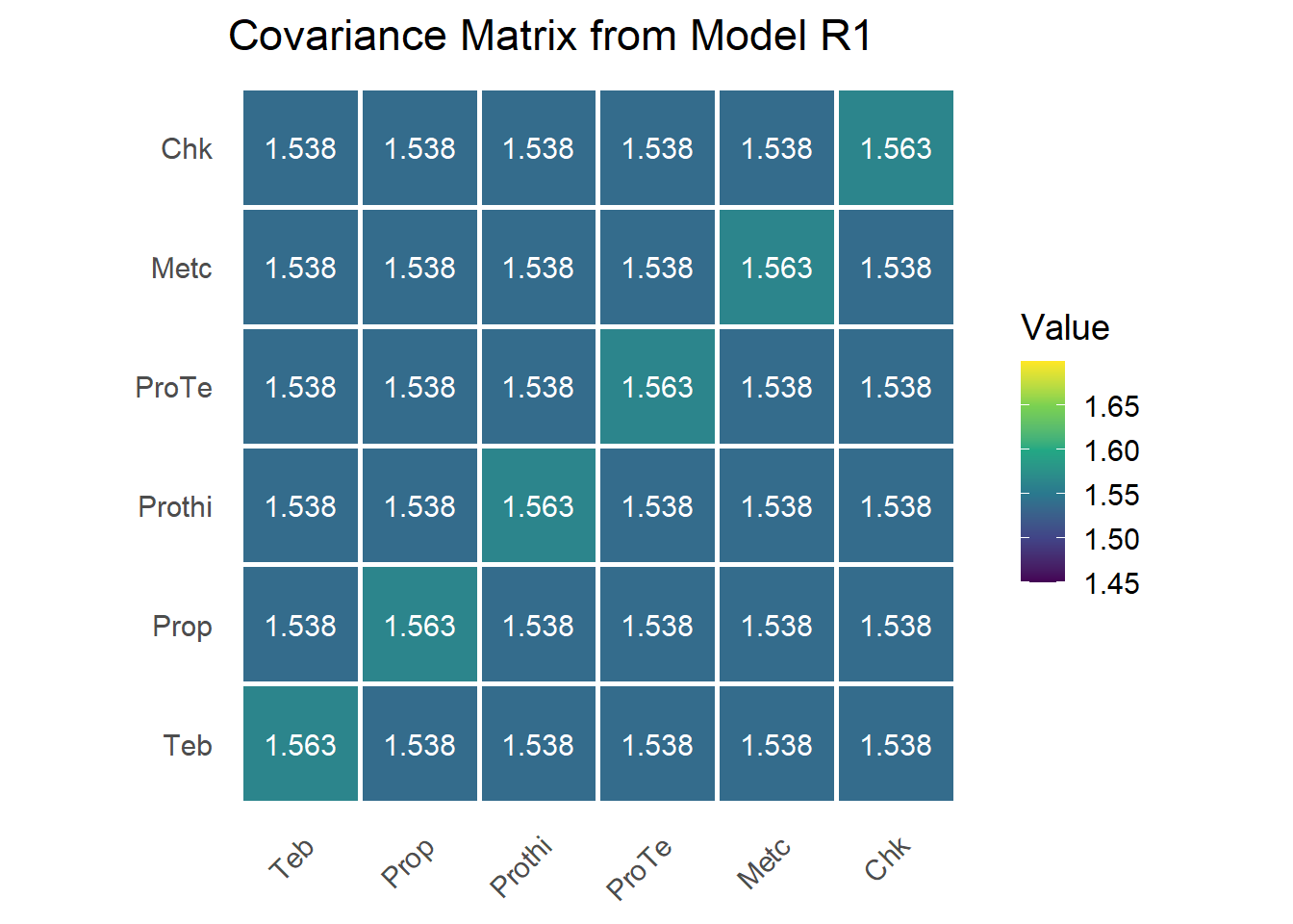
The matrix has equal diagonal entries \(\hat\sigma_\beta^2 + \hat\sigma_u^2\) and equal off-diagonal entries \(\hat\sigma_\beta^2\). The decomposition separates a shared component (\(\sigma_\beta^2\), common to all treatments in a study) from a treatment-specific deviation (\(\sigma_u^2\)). Constant variance plus constant covariance is the signature of compound symmetry.
Treatment predictions and standard errors
predict(mod.r1, classify = "trt", sed = TRUE, vcov = TRUE, trace = FALSE)$pvals##
## Notes:
## [0;34m- The predictions are obtained by averaging across the hypertable
## calculated from model terms constructed solely from factors in
## the averaging and classify sets.
## - Use 'average' to move ignored factors into the averaging set.
## - The ignored set: trial
## [0m
## trt predicted.value std.error status
## 1 Teb 3.807871 0.1079718 Estimable
## 2 Prop 3.732877 0.1108996 Estimable
## 3 Prothi 3.962304 0.1109909 Estimable
## 4 ProTe 3.966229 0.1092001 Estimable
## 5 Metc 3.969550 0.1092708 Estimable
## 6 Chk 3.533565 0.1079718 EstimableThese reproduce the SAS results. Note that the treatment means remain BLUEs (treatment is fixed), but the study and interaction effects \(h_{ij}\) are now BLUPs: shrunken predictions whose contribution to the treatment means recovers interstudy information.
Model R2: heterogeneous compound symmetry
Model R2 keeps the single correlation of CS but lets each treatment have its own variance. This is heterogeneous compound symmetry (CSH):
\[ \operatorname{var}(h_{ij}) = \sigma_{\tau(j)}^2, \qquad \operatorname{cov}(h_{ij}, h_{ij'}) = \rho\,\sigma_{\tau(j)}\,\sigma_{\tau(j')}. \]
A single correlation \(\rho\) links all treatments, but the diagonal is now free. It is implemented with corh(trt):trial.
mod.r2 <- asreml(
  fixed  = yield ~ trt,
  random = ~ corh(trt):trial,                     # heterogeneous CS: free variances, one rho
  weights = "wtyld",
  data    = dat,
  family  = asr_gaussian(dispersion = 1),
  maxiter = 200,
  na.action = na.method(x = "omit", y = "omit"),
  trace   = FALSE
)
Variance component estimates
sum.r2 <- summary(mod.r2)$varcomp; sum.r2## component std.error z.ratio bound %ch
## trt:trial!trt!cor 0.9845368 0.002722033 361.691658 U 0.0
## trt:trial!trt_Teb 1.5430249 0.190560380 8.097302 P 0.0
## trt:trial!trt_Prop 1.5353601 0.200817650 7.645543 P 0.0
## trt:trial!trt_Prothi 1.5423651 0.204580806 7.539149 P 0.1
## trt:trial!trt_ProTe 1.5165437 0.192193963 7.890694 P 0.1
## trt:trial!trt_Metc 1.4375122 0.183292345 7.842729 P 0.1
## trt:trial!trt_Chk 1.6763459 0.207330711 8.085372 P 0.0
## units!R 1.0000000 NA NA F 0.0With six treatments the model estimates six treatment-specific variances (rows ending in trt_...), one shared correlation \(\hat\rho\) (the row ending in cor), and the fixed residual variance. CSH generalizes the equal-variance assumption of CS while retaining a single, interpretable correlation across treatments, so it adds \(m - 1\) parameters relative to CS (seven non-residual parameters here versus two).
The G matrix
We rebuild \(\mathbf{G}\) from the variances and the shared correlation, \(\mathbf{G} = \mathbf{D}^{1/2}\mathbf{C}\mathbf{D}^{1/2}\), where \(\mathbf{D} = \operatorname{diag}(\sigma_{\tau(j)}^2)\) and \(\mathbf{C}\) is a correlation matrix with \(\rho\) off the diagonal.
variances <- sum.r2[!grepl("(cor|R)$", rownames(sum.r2)), 1]
rho       <- sum.r2[grepl("cor$", rownames(sum.r2)), 1]
G <- diag(1, n_trt)
G[upper.tri(G)] <- rho
G[lower.tri(G)] <- t(G)[lower.tri(G)]
G <- diag(sqrt(variances)) %*% G %*% diag(sqrt(variances))
rownames(G) <- colnames(G) <- trt_levels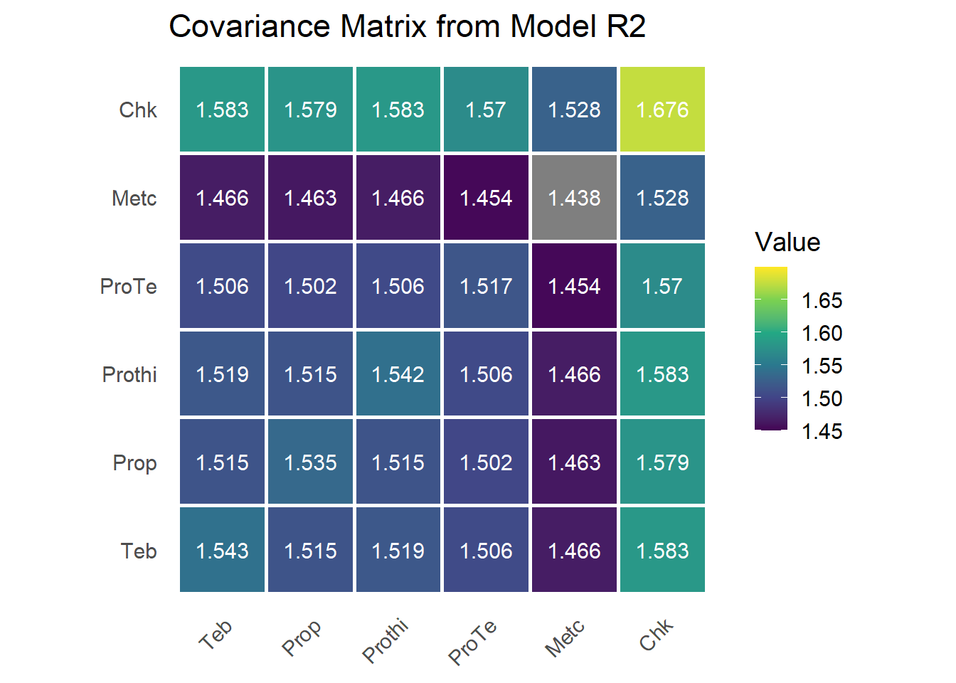
The diagonal now varies by treatment, while the correlation that ties treatments together is constant. CSH is the natural step up from CS when treatments differ in stability but their pairwise relationships are roughly uniform.
Treatment predictions and standard errors
predict(mod.r2, classify = "trt", sed = TRUE, vcov = TRUE, trace = FALSE)$pvals##
## Notes:
## [0;34m- The predictions are obtained by averaging across the hypertable
## calculated from model terms constructed solely from factors in
## the averaging and classify sets.
## - Use 'average' to move ignored factors into the averaging set.
## - The ignored set: trial
## [0m
## trt predicted.value std.error status
## 1 Teb 3.806563 0.1072693 Estimable
## 2 Prop 3.732439 0.1098537 Estimable
## 3 Prothi 3.964428 0.1102102 Estimable
## 4 ProTe 3.966996 0.1075672 Estimable
## 5 Metc 3.971398 0.1048453 Estimable
## 6 Chk 3.537911 0.1117421 EstimableThese again match the SAS output.
Model R3: unstructured covariance
Model R3 places no constraints on \(\mathbf{G}\). Every treatment has its own variance and every pair its own covariance:
\[ \mathbf{G} = \boldsymbol{\Sigma}_{\text{UN}}, \qquad g_{jj'} \text{ free for all } j \le j'. \]
This unstructured (UN) form is the most flexible and the most demanding, with \(m(m+1)/2 = 21\) free covariance parameters for six treatments. It is implemented with us(trt):trial.
mod.r3 <- asreml(
  fixed  = yield ~ trt,
  random = ~ us(trt):trial,                        # unstructured: every variance and covariance free
  weights = "wtyld",
  data    = dat,
  family  = asr_gaussian(dispersion = 1),
  maxiter = 100,
  na.action = na.method(x = "omit", y = "omit"),
  trace = FALSE
)

mod.r3 <- update.asreml(mod.r3)                   # one extra round of REML to reach convergence
mod.r3 <- update.asreml(mod.r3)
mod.r3 <- update.asreml(mod.r3)
The unstructured model converges slowly on this network and can be sensitive to starting values (which we did not specify here, but could naturally be the case).
Variance component estimates
sum.r3 <- summary(mod.r3)$varcomp; sum.r3## component std.error z.ratio bound %ch
## trt:trial!trt_Teb:Teb 1.534299 0.1894087 8.100465 ? 0
## trt:trial!trt_Prop:Teb 1.522754 0.1897824 8.023683 ? 0
## trt:trial!trt_Prop:Prop 1.540293 0.1983300 7.766314 ? 0
## trt:trial!trt_Prothi:Teb 1.511777 0.1892854 7.986761 ? 0
## trt:trial!trt_Prothi:Prop 1.512370 0.1919324 7.879702 ? 0
## trt:trial!trt_Prothi:Prothi 1.528648 0.1989188 7.684782 ? 0
## trt:trial!trt_ProTe:Teb 1.514823 0.1880823 8.054048 ? 0
## trt:trial!trt_ProTe:Prop 1.503421 0.1897357 7.923764 ? 0
## trt:trial!trt_ProTe:Prothi 1.525460 0.1919241 7.948247 ? 0
## trt:trial!trt_ProTe:ProTe 1.533252 0.1937005 7.915582 ? 0
## trt:trial!trt_Metc:Teb 1.472498 0.1826934 8.059945 ? 0
## trt:trial!trt_Metc:Prop 1.476620 0.1854098 7.964088 ? 0
## trt:trial!trt_Metc:Prothi 1.486025 0.1862295 7.979533 ? 0
## trt:trial!trt_Metc:ProTe 1.480920 0.1854530 7.985419 ? 0
## trt:trial!trt_Metc:Metc 1.446315 0.1828574 7.909525 ? 0
## trt:trial!trt_Chk:Teb 1.580484 0.1952287 8.095554 ? 0
## trt:trial!trt_Chk:Prop 1.587587 0.1979974 8.018223 ? 0
## trt:trial!trt_Chk:Prothi 1.556287 0.1964013 7.924017 ? 0
## trt:trial!trt_Chk:ProTe 1.540363 0.1938824 7.944832 ? 0
## trt:trial!trt_Chk:Metc 1.518949 0.1897416 8.005355 ? 0
## trt:trial!trt_Chk:Chk 1.674339 0.2065604 8.105809 ? 0
## units!R 1.000000 NA NA F 0The unstructured model estimates 6 treatment variances, 15 treatment-by-treatment covariances, and the fixed residual, for 21 free covariance parameters. It is the saturated covariance model and imposes no assumptions on \(\mathbf{G}\), which makes it a useful upper reference for how much structure the data can support.
The G matrix
G <- matrix(0, n_trt, n_trt)
G[upper.tri(G, diag = TRUE)] <- sum.r3[grep("trt", rownames(sum.r3)), 1]
G[lower.tri(G, diag = FALSE)] <- t(G)[lower.tri(t(G), diag = FALSE)]
rownames(G) <- colnames(G) <- trt_levels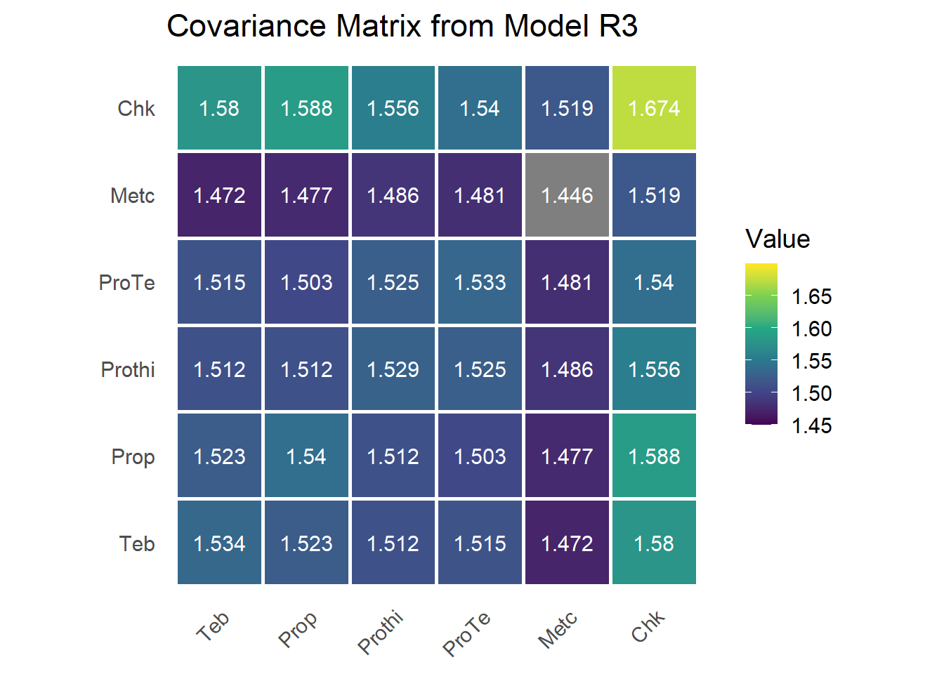
The estimated \(\mathbf{G}\) closely matches the SAS output from the original manuscript.
Treatment predictions and standard errors
predict(mod.r3, classify = "trt", sed = TRUE, vcov = TRUE, trace = FALSE)$pvals##
## Notes:
## [0;34m- The predictions are obtained by averaging across the hypertable
## calculated from model terms constructed solely from factors in
## the averaging and classify sets.
## - Use 'average' to move ignored factors into the averaging set.
## - The ignored set: trial
## [0m
## trt predicted.value std.error status
## 1 Teb 3.807709 0.1069374 Estimable
## 2 Prop 3.734442 0.1093408 Estimable
## 3 Prothi 3.954652 0.1087683 Estimable
## 4 ProTe 3.979865 0.1080307 Estimable
## 5 Metc 3.985435 0.1048532 Estimable
## 6 Chk 3.535294 0.1116977 EstimableTreatment means and standard errors are very close to the SAS-based analysis, with small numerical differences from implementation details.
Model R4: first-order factor analytic (FA1)
The simple structures (R1, R2) may underfit, while the unstructured model (R3) spends 21 parameters and can overfit a sparse network. Factor-analytic (FA) models occupy the middle ground. They approximate \(\mathbf{G}\) with a low-rank term plus a diagonal, which captures the dominant covariance pattern with far fewer parameters. The FA approach was introduced for genotype-by-environment data by Piepho (1997) and developed by Smith, Cullis, and Thompson and others; the original manuscript applies it to NMA.
A first-order factor analytic structure writes
\[ \mathbf{G} = \boldsymbol{\lambda}\boldsymbol{\lambda}^\top + \boldsymbol{\Psi}, \qquad g_{jj} = \lambda_j^2 + \psi_j, \qquad g_{jj'} = \lambda_j \lambda_{j'}, \]
where \(\boldsymbol{\lambda} = (\lambda_1, \dots, \lambda_m)^\top\) are the treatment loadings on a single latent factor, and \(\boldsymbol{\Psi} = \operatorname{diag}(\psi_1, \dots, \psi_m)\) holds the treatment-specific (uniqueness) variances. The shared latent factor generates all covariances, so a treatment’s behavior across studies is summarized by how strongly it loads on one common dimension. It is implemented with fa(trt, 1):trial.
mod.r4 <- asreml(
  fixed  = yield ~ trt,
  random = ~ fa(trt, 1):trial,                     # one latent factor + diagonal uniqueness
  weights = "wtyld",
  family  = asr_gaussian(dispersion = 1),
  data    = dat,
  na.action = na.method(x = "omit", y = "omit"),
  trace   = FALSE
)
mod.r4 <- update.asreml(mod.r4)                     # extra REML round for convergence
Variance component estimates
sum.r4 <- summary(mod.r4)$varcomp; sum.r4## component std.error z.ratio bound %ch
## fa(trt, 1):trial!Teb!var 0.0207547924 0.006873262 3.0196421 P 0.0
## fa(trt, 1):trial!Prop!var 0.0234861593 0.010488692 2.2391886 P 0.0
## fa(trt, 1):trial!Prothi!var 0.0000000000 NA NA F NA
## fa(trt, 1):trial!ProTe!var 0.0190031077 0.007254230 2.6195898 P 0.0
## fa(trt, 1):trial!Metc!var 0.0007040128 0.004456461 0.1579758 P 0.2
## fa(trt, 1):trial!Chk!var 0.0596499167 0.011548078 5.1653547 P 0.0
## fa(trt, 1):trial!Teb!fa1 1.2332963001 0.046228188 26.6784478 P 0.0
## fa(trt, 1):trial!Prop!fa1 1.2330379064 0.051543839 23.9221203 P 0.0
## fa(trt, 1):trial!Prothi!fa1 1.2452533930 0.047978708 25.9542919 P 0.0
## fa(trt, 1):trial!ProTe!fa1 1.2266131750 0.046834790 26.1902140 P 0.0
## fa(trt, 1):trial!Metc!fa1 1.2045660630 0.043815020 27.4920809 P 0.0
## fa(trt, 1):trial!Chk!fa1 1.2669038469 0.048731932 25.9974067 P 0.0
## units!R 1.0000000000 NA NA F 0.0The model reports six factor loadings (rows ending in fa1), six treatment-specific uniqueness variances (rows ending in var), and the fixed residual. That is \(2m = 12\) covariance parameters: fewer than the 21 of the unstructured model, and more than the seven of CSH, which places FA1 squarely between the two in flexibility.
The G matrix
We reconstruct \(\mathbf{G}\) from the loadings and uniquenesses. A singular value decomposition rotates the loadings to a canonical orientation (the sign flip makes the dominant loading positive), then \(\mathbf{G} = \boldsymbol{\lambda}^\star \boldsymbol{\lambda}^{\star\top} + \boldsymbol{\Psi}\).
fa1.loadings <- sum.r4[endsWith(rownames(sum.r4), "fa1"), 1]
mat.loadings <- as.matrix(cbind(fa1.loadings))
svd.mat.loadings <- svd(mat.loadings)
mat.loadings.star <- mat.loadings %*% svd.mat.loadings$v * -1   # rotate to canonical sign
colnames(mat.loadings.star) <- c("fa1")
psi <- as.matrix(diag(sum.r4[endsWith(rownames(sum.r4), "var"), 1]))
lamb_lamb_t <- mat.loadings.star %*% t(mat.loadings.star)
G <- lamb_lamb_t + psi
rownames(G) <- colnames(G) <- trt_levels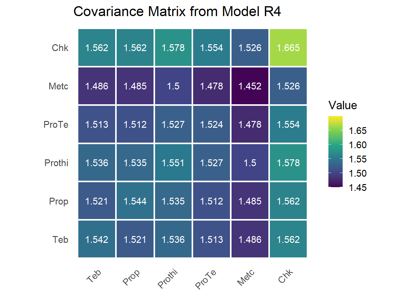
Diagonal entries are total variances (\(\lambda_j^2 + \psi_j\)); off-diagonals are the covariances implied by shared loading on the single latent dimension (\(\lambda_j \lambda_{j'}\)). The whole covariance pattern is thus generated by one factor plus treatment-specific noise.
Treatment predictions and standard errors
predict(mod.r4, classify = "trt", sed = TRUE, vcov = TRUE, trace = FALSE)$pvals##
## Notes:
## [0;34m- The predictions are obtained by averaging across the hypertable
## calculated from model terms constructed solely from factors in
## the averaging and classify sets.
## - Use 'average' to move ignored factors into the averaging set.
## - The ignored set: trial
## [0m
## trt predicted.value std.error status
## 1 Teb 3.807798 0.1072221 Estimable
## 2 Prop 3.738126 0.1100908 Estimable
## 3 Prothi 3.955384 0.1091113 Estimable
## 4 ProTe 3.968101 0.1077004 Estimable
## 5 Metc 3.976248 0.1047761 Estimable
## 6 Chk 3.537135 0.1113974 EstimableThe FA1 means and standard errors are close to the SAS-based analysis, with small numerical differences.
Model R5: second-order factor analytic (FA2)
Model R5 adds a second latent factor:
\[ \mathbf{G} = \boldsymbol{\Lambda}\boldsymbol{\Lambda}^\top + \boldsymbol{\Psi}, \qquad \boldsymbol{\Lambda} = [\boldsymbol{\lambda}_1\ \boldsymbol{\lambda}_2], \]
where \(\boldsymbol{\Lambda}\) is \(m \times 2\). A second dimension captures covariance patterns that a single factor cannot, while still costing fewer parameters than the unstructured model. It is implemented with fa(trt, 2):trial.
mod.r5 <- asreml(
  fixed  = yield ~ trt,
  random = ~ fa(trt, 2):trial,                     # two latent factors + diagonal uniqueness
  weights = "wtyld",
  family  = asr_gaussian(dispersion = 1),
  data    = dat,
  na.action = na.method(x = "omit", y = "omit"),
  trace   = FALSE
)
mod.r5 <- update.asreml(mod.r5)
Variance component estimates
sum.r5 <- summary(mod.r5)$varcomp; sum.r5## component std.error z.ratio bound %ch
## fa(trt, 2):trial!Teb!var 0.014399834 0.006010461 2.39579513 P 0.0
## fa(trt, 2):trial!Prop!var 0.016230094 0.009689854 1.67495756 P 0.0
## fa(trt, 2):trial!Prothi!var 0.000000000 NA NA F NA
## fa(trt, 2):trial!ProTe!var 0.002392063 0.006898018 0.34677540 P 0.1
## fa(trt, 2):trial!Metc!var 0.003520856 0.004823912 0.72987564 P 0.0
## fa(trt, 2):trial!Chk!var 0.001379427 0.018633980 0.07402753 P 0.3
## fa(trt, 2):trial!Teb!fa1 1.232504245 0.044682189 27.58379304 P 0.0
## fa(trt, 2):trial!Prop!fa1 1.231837892 0.049159320 25.05807449 P 0.0
## fa(trt, 2):trial!Prothi!fa1 1.231338194 0.048496754 25.39011583 P 0.0
## fa(trt, 2):trial!ProTe!fa1 1.222544048 0.046465128 26.31100149 P 0.0
## fa(trt, 2):trial!Metc!fa1 1.199053959 0.043428730 27.60969417 P 0.0
## fa(trt, 2):trial!Chk!fa1 1.281841982 0.047645383 26.90380244 P 0.0
## fa(trt, 2):trial!Teb!fa2 0.000000000 NA NA F NA
## fa(trt, 2):trial!Prop!fa2 -0.036711099 0.038797425 -0.94622515 P 0.0
## fa(trt, 2):trial!Prothi!fa2 0.124818564 0.032007761 3.89963434 P 0.0
## fa(trt, 2):trial!ProTe!fa2 0.173897080 0.034970372 4.97269753 P 0.0
## fa(trt, 2):trial!Metc!fa2 0.090695492 0.027525036 3.29501812 P 0.0
## fa(trt, 2):trial!Chk!fa2 -0.172290283 0.047570236 -3.62180850 P 0.0
## units!R 1.000000000 NA NA F 0.0length(sum.r5$component)## [1] 19The model reports six first-order loadings (fa1), six second-order loadings (fa2), six uniqueness variances (var), and the fixed residual. The second factor explains additional treatment-by-study structure that one dimension misses, while remaining more parsimonious than the unstructured model. The printed length() gives the exact parameter count for this fit.
The G matrix
fa1.loadings <- sum.r5[endsWith(rownames(sum.r5), "fa1"), 1]
fa2.loadings <- sum.r5[endsWith(rownames(sum.r5), "fa2"), 1]
mat.loadings <- as.matrix(cbind(fa1.loadings, fa2.loadings))
svd.mat.loadings <- svd(mat.loadings)
mat.loadings.star <- mat.loadings %*% svd.mat.loadings$v * -1
colnames(mat.loadings.star) <- c("fa1", "fa2")
psi <- as.matrix(diag(sum.r5[endsWith(rownames(sum.r5), "var"), 1]))
lamb_lamb_t <- mat.loadings.star %*% t(mat.loadings.star)
G <- lamb_lamb_t + psi
rownames(G) <- colnames(G) <- trt_levels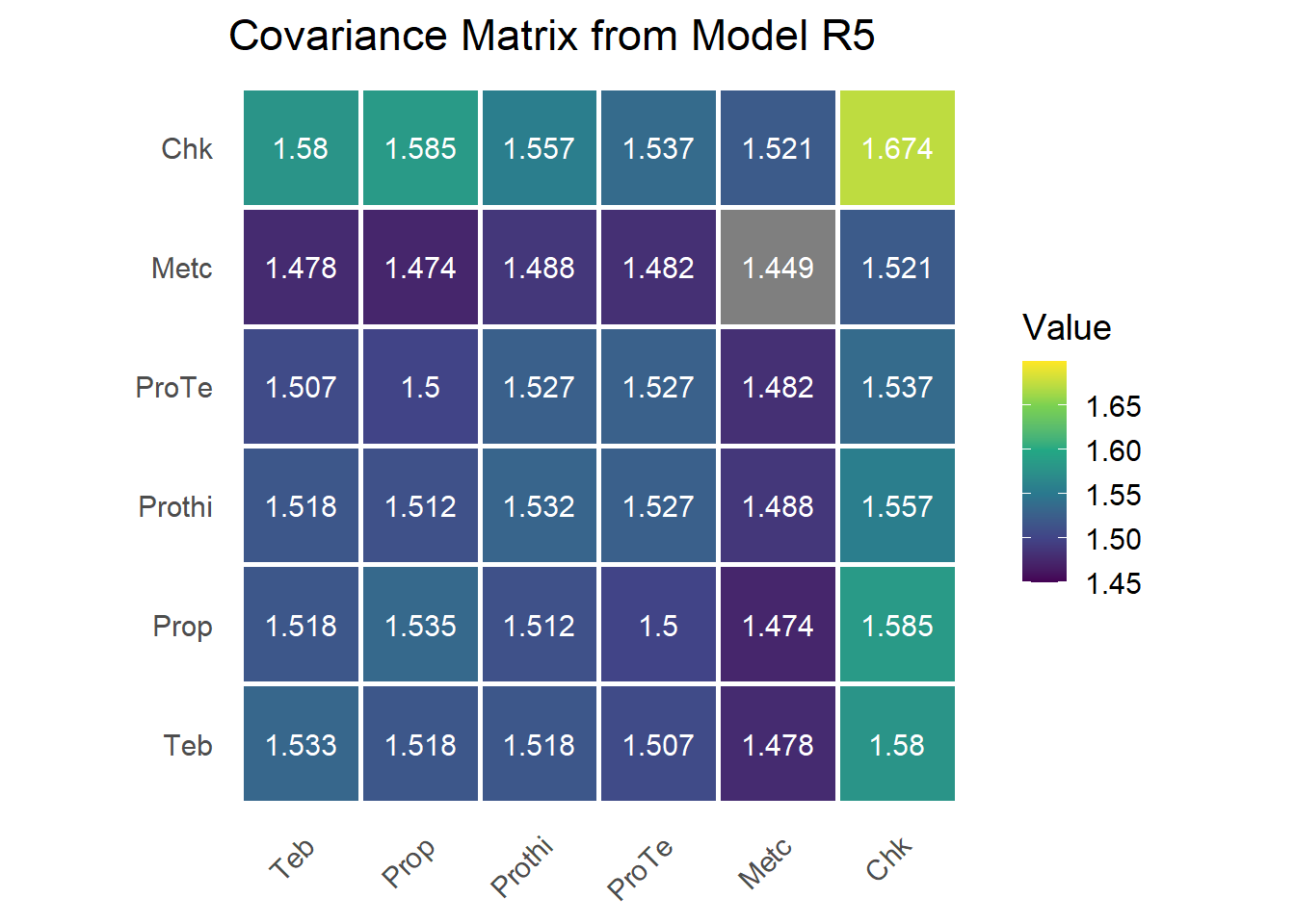
Treatment predictions and standard errors
predict(mod.r5, classify = "trt", sed = TRUE, vcov = TRUE, trace = FALSE)$pvals##
## Notes:
## [0;34m- The predictions are obtained by averaging across the hypertable
## calculated from model terms constructed solely from factors in
## the averaging and classify sets.
## - Use 'average' to move ignored factors into the averaging set.
## - The ignored set: trial
## [0m
## trt predicted.value std.error status
## 1 Teb 3.807799 0.1069134 Estimable
## 2 Prop 3.731821 0.1092218 Estimable
## 3 Prothi 3.955729 0.1087187 Estimable
## 4 ProTe 3.978682 0.1079482 Estimable
## 5 Metc 3.984402 0.1048775 Estimable
## 6 Chk 3.535239 0.1116943 EstimableComparing Models R1 through R5
All five random-study models share the same fixed effects (yield ~ trt), so their REML log-likelihoods and AIC values are directly comparable.
mods.asr <- list(mod.r1, mod.r2, mod.r3, mod.r4, mod.r5)
asremlPlus::infoCriteria(mods.asr)
## fixedDF varDF NBound AIC BIC loglik
## 1 0 2 1 -414.6803 -406.0532 209.3401
## 2 0 7 1 -414.8112 -384.6163 214.4056
## 3 0 21 1 -457.8641 -367.2796 249.9321
## 4 0 11 2 -431.6603 -384.2113 226.8301
## 5 0 16 3 -460.6783 -391.6616 246.3392Model R5 (FA2) attains the lowest AIC. It matches or exceeds the log-likelihood of the unstructured model while estimating fewer parameters, which is the parsimony that AIC rewards. The AIC and log-likelihood values differ slightly from the original manuscript because their figures use ML estimation for some comparisons while these use REML; the two scales are not directly comparable. Both approaches nonetheless select R5 as the best random-effects model, which says the treatment-by-study covariance in this network is well summarized by two latent dimensions.
Final remarks
This post walked through a graded sequence of NMA models for multi-treatment trial data. The fixed-study models start from a single between-study variance (F1) and then allow treatment-specific variances (F2). The random-study models recover interstudy information and build up covariance structure: compound symmetry (R1), heterogeneous compound symmetry (R2), the unstructured form (R3), and the factor-analytic forms (R4 and R5).
The pattern across the random-study models is the familiar bias-variance trade in covariance modeling. CS and CSH are stable but rigid. The unstructured model is maximally flexible but parameter-hungry and unstable on a sparse network. The factor-analytic models capture most of the between-study covariance with a handful of latent dimensions, and FA2 gave the best fit here by AIC. Latent factors are an effective way to describe treatment-by-study interaction in networked agronomic data, just as they are for genotype-by-environment data.
This framework suits agricultural research where treatments are replicated unevenly across locations and where borrowing strength across a network sharpens inference. Open-source packages such as metafor, nlme, and lme4breeding can fit related models, with the residual-scale caveat noted above for the lme4-based engines; a later post will compare them directly. All models here used summary-level data, which mirrors what published field trials typically report. A future post will extend these methods to individual plot-level data, which opens the door to spatial structure, trial-specific errors, and plot-level covariates.

Vini Garnica
Assistant Professor
Quantitative plant pathologist developing data-driven tools for disease prediction and crop management.