Data imputation for designed experiments
Whenever I get my hands on a new dataset (regardless of data being collected by me or someone else) and I find missing data, and that makes me frustrated. And do you know when that happens?? Almost all the time.
A variety of errors can happen when carrying experiments. For example, in the field, a plot may be damaged by tractor track or deer. In the lab, we may drop off a Petri plate or touch the media with nonsterile tool. The standard approach for data analysis when missing data occurs is to delete or omit them from analysis and the inclination to delete missing data is understandable. Apart from the technical difficulties imposed by the missing data, its occurrence has long been considered a sign of sloppy research. But, missing data are there, whether you like it or not, so imputation of missing values may be valuable in data analysis.
In this exercise, we’ll be evaluating imputation methods for a continuous outcome arising from designed experiments. This type of simulation is one of my favorites and is something I am interested in as part of my own research. For that reason I decided to make the code publicly available in case others are also curious about the performance of R packages for data imputation and/or have suggestions on how to improve what is displayed here. Note that the majority of examples on the web encompasses observational data, so this exercise may be somewhat interesting…
The exercise is going to be split in two parts. The first one, we will be looking at imputation techniques for experiments carried out as randomized complete block design (RCBD) where the missingness mechanism is random and no covariate is added into the imputation algorithms. The second part of the exercise will be conducted in a similar manner with the exception that a covariate at the site level will be included in the imputation mechanism. This covariate may be something like rainfall over grain filling period or nitrogen levels at the site level, instead of the plot level.
Loading packages
library(pacman)

p_load(lme4,
       kableExtra,
       missForest,
       naniar,
       mice,
       miceadds,
       VIM,
       mixgb,
       tidyverse)
The very first step is to generate data from trials arranged in RCBD. The number of treatment and blocks will be the same across trials, 8 and 4, respectively, for a total of 32 observations per trial. In the world of simulation we have access to both the true and imputed values, so an obvious way to quantify the quality of a method is to see how well it can recreate the true data.
Obs.: Feel free to play with the code below to understand what’s going on during the simulation.
Before we move on, please, check this blog to learn about MCAR, MAR, and MNAR. These are not a traditional dish of the Brazilian cuisine, but instead the terminology describing the mechanism of missing data. They can be:
- Completely at random (MCAR)
- Missing at random (MAR)
- Missing not at random (MNAR)
Learning about these mechanisms is important because that will have implication on the techniques used for imputation. Yet, it is often difficult to detect the missing values mechanism in practice exactly, because this would require the knowledge of the missing values themselves. That’s why simulation is handy…
Part 1: MCAR imputation of response variable in designed experiments
Generating data
set.seed(2022)
{
  trials<-6
  data<-vector("list", trials)
  mylF<-vector("list", trials)
  blocklF<-vector("list", trials)
  Z<-vector("list", trials)
  bZ<-vector("list", trials)
  b.trt<-vector("list", trials)
  b.block<-vector("list", trials)


  for(i in 1:trials){
      data[[i]]<- data.frame(expand.grid(trt=1:8,block=1:4)) # create a data frame with 8 treatments and 4 blocks
      data[[i]]$site=i  # add a site id variable
      data[[i]]$y <- sample(30:70,1) + rnorm(nrow(data[[i]]),sd=8) # generate a random sample from 30 to 70 and add error Y~N(0,64)

      myformula <- "y ~ block + (1|trt)"
      mylF[[i]] <- lFormula(eval(myformula), data = data[[i]]) # extract design matrix
      Z[[i]] <- mylF[[i]]$reTrms$Zt %>% as.matrix() %>% t()   # extract design matrix
      b.trt[[i]] <- rnorm(8, 2, sd=2)  # add a treatment effect. Note that effect varies between treatments but it is constant between replicates and random across trials

      myformula <- "y ~ (1|block)"  # add a block effect
      blocklF[[i]] <- lFormula(eval(myformula), data = data[[i]])
      bZ[[i]] <- blocklF[[i]]$reTrms$Zt %>% as.matrix() %>% t()
      b.block[[i]] <- rnorm(4, 1, sd=0.5)

      data[[i]]$Y <- data[[i]]$y + Z[[i]] %*% b.trt[[i]] + bZ[[i]] %*% b.block[[i]] # add everything together
      data[[i]]<-data.frame(data[[i]])
    }
}
As we can see, the first generated data set has 32 observations, comprising of 8 treatments, 4 blocks, the column site (site identifier), y which is the outcome with no treatment or block effect added, Y which is the outcome after treatment and block effects have been structurally added to each trial. The choice of treatment, block, and overall trial effect sizes simulates, at least partially, some scenarios of yield responses from trials I am used to analyzing. Note that the treatment effect size is the same across all replicates but varies across trials. We have set things up in this way because I believe this would be the most pessimistic scenario, which treatment 1 varies across trials. Do you agree?
data[[1]]## trt block site y Y
## 1 1 1 1 68.02345 72.83317
## 2 2 1 1 65.88010 68.55153
## 3 3 1 1 67.77784 71.13164
## 4 4 1 1 51.17438 56.27865
## 5 5 1 1 70.57995 75.00631
## 6 6 1 1 57.03774 56.94811
## 7 7 1 1 65.38912 69.57787
## 8 8 1 1 55.69978 58.48249
## 9 1 2 1 65.29101 70.54203
## 10 2 2 1 73.32275 76.43549
## 11 3 2 1 66.41765 70.21274
## 12 4 2 1 56.25631 61.80188
## 13 5 2 1 77.11794 81.98561
## 14 6 2 1 87.62045 87.97212
## 15 7 2 1 71.00630 75.63636
## 16 8 2 1 67.81710 71.04112
## 17 1 3 1 63.08412 67.88555
## 18 2 3 1 53.07169 55.73483
## 19 3 3 1 66.00283 69.34833
## 20 4 3 1 70.78151 75.87748
## 21 5 3 1 63.82672 68.24479
## 22 6 3 1 65.49232 65.39439
## 23 7 3 1 54.77697 58.95744
## 24 8 3 1 67.61152 70.38594
## 25 1 4 1 73.38302 77.94689
## 26 2 4 1 60.45917 62.88475
## 27 3 4 1 62.32650 65.43444
## 28 4 4 1 66.54877 71.40719
## 29 5 4 1 63.51244 67.69295
## 30 6 4 1 56.41025 56.07476
## 31 7 4 1 65.74459 69.68749
## 32 8 4 1 72.32717 74.86403Data wrangling and missingness generation
Next, we will be doing some data wrangling and creating a completely random missing pattern (clustered by site of course, although some may say this is not MCAR) in the response variable Y. That means that a treatment is omitted from block 1 but may still be present in blocks 2 and 3. This is important to note as this pattern will not be repeated in the second part of the exercise.
dt = do.call(rbind,data) %>% # combine trials
  select(-y) %>%
  mutate_at(vars(block,trt),as.factor) %>% # format variables (some of the imputation methods below require dt to be numeric)
  unite("block",c(site,block),remove = FALSE) %>% # create unique id for blocks
  mutate(block = as.factor(as.numeric(as.factor(block)))) # create unique id for blocks

dt$Y=round(as.numeric(dt$Y),1)
We will be generating 10%, 20%, and 40% of missing observations per site, randomly performed across treatments. The mechanism for missingness is INDEPENDENT for each missing severity (i.e. 10%, 20%, or 40%). In other words, the missingness is not increasingly added to the previous “treated” dataset. With such design, comparisons BETWEEN missingness severities will be unfair, right? So, we focus on comparing methods within the same missingness severity.
# formula to produce NAs based on site

na.producer = function(dataset,na_percentage){
  dataset %>%
        group_by(site) %>%
        mutate(Y =  replace(Y, sample(row_number(),size = ceiling(na_percentage * n()), replace = FALSE), NA)) %>%  #Create mistiness in the dt by site
        as.data.frame()
}
set.seed(2022)
mis.10 = na.producer(dt,na_percentage = 0.1)
mis.20 = na.producer(dt,na_percentage = 0.2)
mis.40 = na.producer(dt,na_percentage = 0.4)
Checking the number of missing data points
In total, 4, 7 or 8, and 12 or 13 observations are lost at random per site for 10%, 20% and 40% missingness data sets, respectively.
We also can visually explore missing data patterns in this simulated data sets.
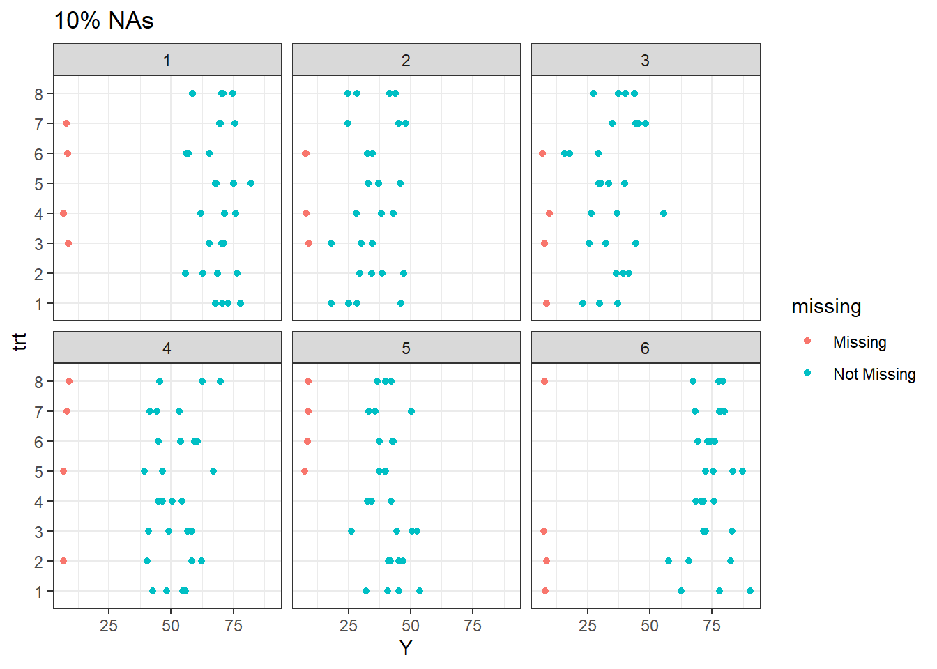
The plot above display the pattern of missingness. Note that for 10% missingness, at site 1, one observation were lost for treatment 7, 6, 4, and 3. The remaining treatments are present.
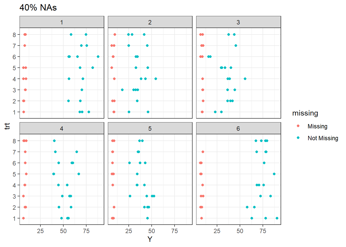
For 40% missingness at site 1, nearly all treatments except 6 have lost one or more observations. All other treatments occur at least once per site.
1) missForest
missForest is a R package used to impute missing values particularly in the case of mixed-type data. It uses a random forest trained on the observed values of a dt matrix to predict the missing values. It can be used to impute continuous and/or categorical dt including complex interactions and non-linear relations. It yields an out-of-bag (OOB) imputation error estimate without the need of a test set or elaborate cross-validation.
Advantages:
- Non-parametric, no assumption about the relationship of the variables
- Can be applied to mixed dt types (numeric and categorical variables)
- No critical assumptions required (aside from the standard assumption of being MAR/MCAR). Check this if you not sure what MAR/MCAR is.
- Robust to noisy dt, especially when compared to KNN
- Excellent predictive power
Disadvantages:
- Imputation time, which is not going to be a big deal here
- Interpretability of random forest. Check this if you not sure what this means.
Imputation is carried out through the following formula:
imp.for.10=missForest(mis.10,maxiter = 20,ntree = 500)imp.for.20=missForest(mis.20,maxiter = 20,ntree = 500)imp.for.40=missForest(mis.40,maxiter = 20,ntree = 500)2) mice
The mice package in R, helps you imputing missing values with plausible data values. These plausible values are drawn from a distribution specifically designed for each missing data point. The package creates multiple imputations (replacement values) for multivariate missing data. The method is based on Fully Conditional Specification, where each incomplete variable is imputed by a separate model. The MICE algorithm can impute mixes of continuous, binary, unordered categorical and ordered categorical dt. MICE operates under the assumption that given the variables used in the imputation procedure, the missing dt are Missing At Random (MAR), which means that the probability that a value is missing depends only on observed values and not on unobserved values
Advantages:
- Each attribute is modeled according to its distribution
- Algorithm can be run multiple times in parallel to obtain m imputed datasets
- Offers a variety of methods for imputation
Disadvantages:
- Assumption that missing values are MAR, which means that its use in a dataset where the missing values are not MAR could generate biased imputations
- Computionally expensive for large data sets
Imputation is carried out through the following formula:
Via 2l.lmer
Setting up the general imputation function based on the linear mixed effects model as implemented in lme4::lmer.
predMatrix = make.predictorMatrix(data = mis.10) # matrix applies for all the missing data sets ()10%, 20%, 40%)
impMethod = make.method(data = mis.10)
impMethod["Y"] = "2l.lmer"

# specify cluster indicator and random effect
predMatrix["site","Y"] = -2 # site needs to be numeric
predMatrix["block","Y"] = 2

# ... specify levels of higher-level variables
level <- character(ncol(mis.10))
names(level) <- colnames(mis.10)

level["block"] <- "site"

# specify cluster indicators (as list)
cluster = list()

cluster[["block"]] = c("site")
cluster[["Y"]] = c("block", "site")
We apply the hierarchical structure in the model and run one iteration for each severity missingness.
imp.lmer.10 = mice(mis.10, method = impMethod, predictorMatrix = predMatrix, maxit = 20,
            m = 1, plevels_id = cluster, variables_levels = level,seed=500)
imp.lmer.20 = mice(mis.20, method = impMethod, predictorMatrix = predMatrix, maxit = 20,
m = 1, plevels_id = cluster, variables_levels = level,seed=500)imp.lmer.40 = mice(mis.40, method = impMethod, predictorMatrix = predMatrix, maxit = 20,
m = 1, plevels_id = cluster, variables_levels = level,seed=500)Via norm.predict
Imputes univariate missing data using the predicted value from a linear regression. Similarly to above, we set the model parameters.
predMatrix = make.predictorMatrix(data = mis.10)
impMethod = make.method(data = mis.10)
impMethod["Y"] = "norm.predict"

# specify cluster indicator
predMatrix["site","Y"] = -2
predMatrix["block","Y"] = 2
imp.norm.pred.10 = mice(mis.10, method = impMethod,predictorMatrix = predMatrix, maxit = 1,seed=500)imp.norm.pred.20 = mice(mis.20, method = impMethod,predictorMatrix = predMatrix, maxit = 1,seed=500)imp.norm.pred.40 = mice(mis.40, method = impMethod,predictorMatrix = predMatrix, maxit = 1,seed=500)3) VIM
VIM introduces new tools for the visualization of missing and/or imputed values, which can be used for exploring the data and the structure of the missing and/or imputed values. Depending on this structure of the missing values, the corresponding methods may help to identify the mechanism generating the missings and allows to explore the data including missing values. In addition, the quality of imputation can be visually explored using various univariate, bivariate, multiple and multivariate plot methods.
Advantages:
- Offers a few methods for data imputation
- Easy model specification
Disadvantages:
- No direct support for longitudinal data
Imputation is carried out through the following formula:
Using a random forest model
imp.ranger.10 = rangerImpute(Y ~ site + trt + block, mis.10)imp.ranger.20 = rangerImpute(Y ~ site + trt + block, mis.20)imp.ranger.40 = rangerImpute(Y ~ site + trt + block, mis.40)Using a regression imputation
imp.reg.10 = regressionImp(Y ~ site + trt + block, mis.10)imp.reg.20 = regressionImp(Y ~ site + trt + block, mis.20)imp.reg.40 = regressionImp(Y ~ site + trt + block, mis.40)4) mixgb
‘mixgb’ is a scalable multiple imputation framework based on XGBoost, bootstrapping and predictive mean matching. The proposed framework is implemented in an R package mixgb. We have shown that our framework obtains less biased estimates and reflects appropriate imputation variability, while achieving high computational efficiency.
Advantages:
- High speed and accuracy
- Efficient for capturing complex structures of large data sets
Imputation is carried out through the following formula:
mixgb.10 = mixgb(data = mis.10, m =1,nrounds = 10)mixgb.20 = mixgb(data = mis.20, m =1,nrounds = 10)mixgb.40 = mixgb(data = mis.40, m =1,nrounds = 10)Results
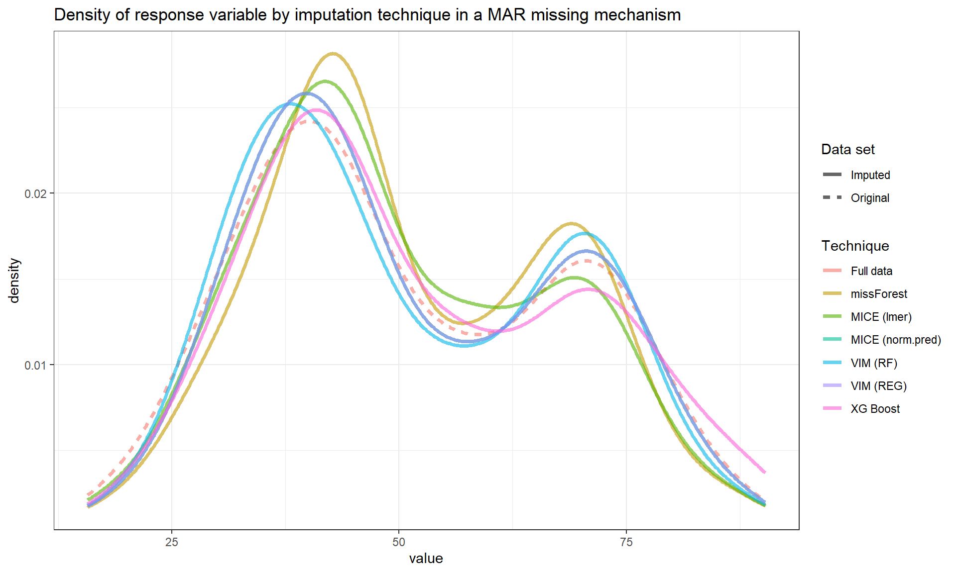
Below we can see the performance of imputation methods via: plot density and RMSE.
Not surprisingly, as the amount of missing data increases, the uncertainty of imputation increases and more extreme values are imputed.
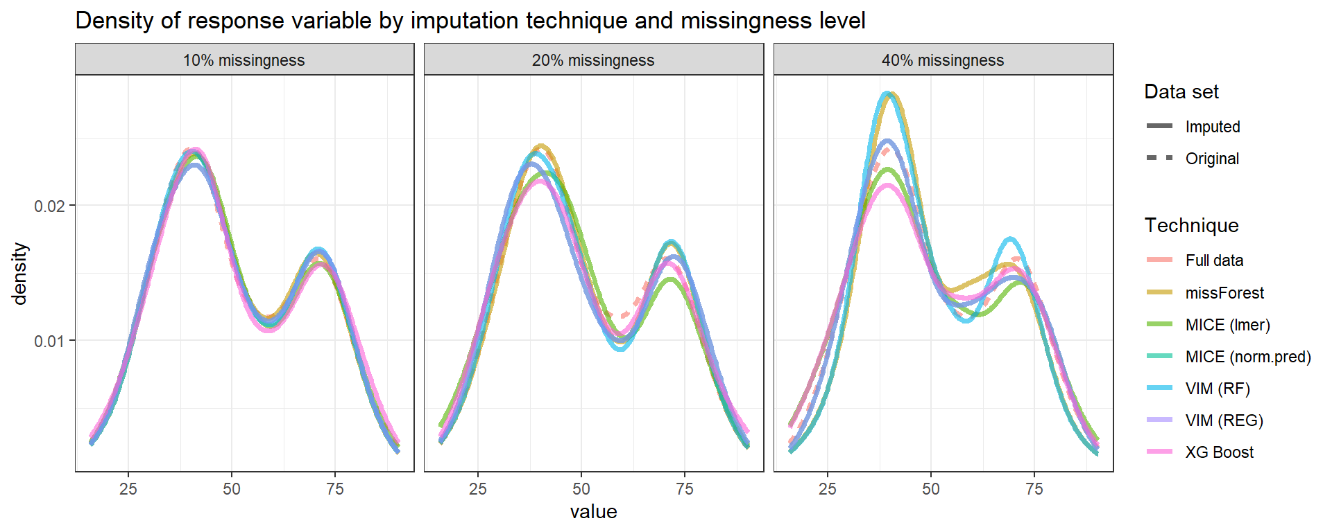
We can see that methods have similar performance under low missingness severity (i.e. 10%) but larger differences arise as more and more data is missing. When accounting for visual differences solely, the imputaion method seems to matter more under higher missigness severity.
RMSE
We know that the minimum RMSE is attained by predicting the missing \(y^{(mis)}_i\) that is closest to the real \(y_i\). The formula to calculate RMSE is:
\[ RMSE = \sqrt{\sum^{n_{mis}}_{i=1}(y^{(mis)}_i-y_i)^2 \over n_{mis}} \] In R, this formula is equivalent to:
rmse = function(imp, mis_dt, truedt) {
  sqrt(sum((imp - truedt)^2)/sum(is.na(mis_dt)))
}
The RMSE values for each method are displayed below.
| 10% | 20% | 40% | |
|---|---|---|---|
| missForest | 9.17 | 7.34 | 8.56 |
| MICE (lmer) | 23.54 | 21.19 | 25.66 |
| MICE (norm.pred) | 9.51 | 9.14 | 8.96 |
| VIM (RF) | 9.18 | 8.25 | 7.88 |
| VIM (REG) | 9.51 | 9.14 | 8.96 |
| XG Boost | 10.95 | 11.28 | 10.75 |
MICE (lmer) seems to have a lower precision compared to other methods using data from this simulated exercise. I imagine some of that is attributed to varying treatment effects across trials (i.e. TRT1 could potentially have the largest effect size in trial 1 and the lowest effect size in trial 2) and the hierarchical structure potentially would under perform in this scenario?
Correlation
Let’s look at the Pearson’s product moment correlation coefficient.| 10% | 20% | 40% | |
|---|---|---|---|
| missForest | 0.84 | 0.88 | 0.87 |
| MICE (lmer) | 0.06 | 0.10 | -0.01 |
| MICE (norm.pred) | 0.84 | 0.87 | 0.86 |
| VIM (RF) | 0.84 | 0.86 | 0.89 |
| VIM (REG) | 0.84 | 0.87 | 0.86 |
| XG Boost | 0.85 | 0.81 | 0.82 |
We observe a low correlation between one of the methods. We could increase the number of trials to 15 or 20 and evaluate the same things but overall, I believe this exercise provides some reasonable comparisons of commonly adopted methods for data imputation in R.
Obs: There has been some critique in the literature related to the adopted evaluation criteria (RMSE and correlation).
Part 2: MAR imputation of response variable in designed experiments WITH covariate at site level.
So far we have only used categorical variables to impute missing data in the continuous outcome response Y. The goal here is to create a covariate at the cluster level (site, in this example) and evaluate its usefulness for imputing Y.
As mentioned before, this would be similar to collecting information at the site level, such as accumulated precipitation during the grain filling period or nitrogen levels at the sites. Overall, adding meaningful covariates in linear regression is an useful technique to reduce the error.
The idea of using a covariate at the site level instead of the plot level is clear. They are more easy to obtain, unless you already are collecting additional information at the plot level. Another reason is that, on average, I have seen a more consistent and sometimes larger effects of site (i.e. environment, location, etc) than a treatment itself in yield responses of row crops such as soybean, corn, and cotton. In other words, whenever I am evaluating multi-environment trials, location (and its hidden factors) is usually number 1 parameter explaining yield variability. So, let’s jump in the analysis and see how the performance changes as a covariate is added.
In the simulation process, the covariate will need to be associated (positively or negatively, linearly or not) with Y by site. I believe we can achieve that in the following manner.
set.seed(2022)

rain=dt %>%
  group_by(site) %>%
  summarize(m_Y= mean(Y)) %>%
  mutate(rain = m_Y*10 + rnorm(6,0,120))

rain
## # A tibble: 6 × 3
## site m_Y rain
## <int> <dbl> <dbl>
## 1 1 68.8 796.
## 2 2 35.4 213.
## 3 3 35.6 249.
## 4 4 51.3 339.
## 5 5 39.9 360.
## 6 6 74.2 394.Basically, we created a covariate (rain) at the site level that is associated with Y. The rain variable is not strongly associated with Y, which makes sense, as we know, other factors also influence yield. Note for example, site 1, 2, and 5 have comparable yield levels despite different levels of precipitation.
dt= left_join(dt,rain %>% select(-m_Y),by="site")Now, we repeat all the steps above, except that the rain covariate is not added to the model.
Missingness generation
We also will change the mechanism of data missingness. Before, observations were lost at random, but now we will add a structure to data deletion. We will omit specific treatments from half of the sites and other treatments from the remaining ones.
In other words, treatments 1 and 2 will be removed from the first three sites and similarly, treatments 7 and 8 will be removed from sites 5 and 6, simulating a scenario of MAR missing mechanism.
# formula to produce NAs based on site and treatment

mis = dt %>%
  mutate(Y = replace(Y, site %in% c(1:3) & trt %in% c(1:2),NA)) %>%
  mutate(Y = replace(Y, site %in% c(5:6) & trt %in% c(7:8),NA))
Checking the number of missing data points
Let’s take a look on the missing data.
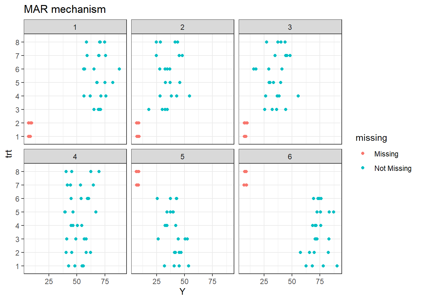
As it was said before, treatments 1 and 2 are missing in site 1, 2, and 3. Additionally, treatments 7 and 8 are missing in sites 5 and 6.
1) missForest
Imputation is carried out through the following formula:
imp.for=missForest(mis,maxiter = 20,ntree = 500)2) mice
Imputation is carried out through the following formula:
Via 2l.lmer
predMatrix = make.predictorMatrix(data = mis)
impMethod = make.method(data = mis)
impMethod["Y"] = "2l.lmer"

# specify cluster indicator and random effect
predMatrix["site","Y"] = -2 # site needs to be numeric
predMatrix["block","Y"] = 2

# ... specify levels of higher-level variables
level <- character(ncol(mis))
names(level) <- colnames(mis)

level["block"] <- "site"
level["rain"] <- "site"

# specify cluster indicators (as list)
cluster = list()

cluster[["block"]] = c("site")
cluster[["Y"]] = c("block", "site")
cluster[["rain"]] = c("site")
We apply the hierarchical structure in the model and run one iteration for each severity missingness.
imp.lmer = mice(mis, method = impMethod, predictorMatrix = predMatrix, maxit = 20,
            m = 1, plevels_id = cluster, variables_levels = level,seed=500)
Using norm.predict
predMatrix = make.predictorMatrix(data = mis)
impMethod = make.method(data = mis)
impMethod["Y"] = "norm.predict"

# specify cluster indicator
predMatrix["site","Y"] = -2
predMatrix["block","Y"] = 2
imp.norm.pred = mice(mis, method = impMethod,predictorMatrix = predMatrix, maxit = 1,seed=500)3) VIM
Imputation is carried out through the following formula:
Using a random forest model
imp.ranger = rangerImpute(Y ~ site + trt + block + rain, mis)Using a regression imputation
imp.reg = regressionImp(Y ~ site + trt + block + rain, mis)4) mixgb
Imputation is carried out through the following formula:
mixgb = mixgb(data = mis, m =1,nrounds = 10)Results
RMSE
The RMSE values for each method are displayed below.
| RMSE | |
|---|---|
| missForest | 9.49 |
| MICE (lmer) | 23.31 |
| MICE (norm.pred) | 7.14 |
| VIM (RF) | 6.94 |
| VIM (REG) | 7.14 |
| XG Boost | 10.37 |
The MICE (lmer) seems to be less precise compared to other methods in this simulated example.
Correlation
Let’s look at the Pearson’s product moment correlation coefficient.| x | |
|---|---|
| missForest | 0.93 |
| MICE (lmer) | 0.02 |
| MICE (norm.pred) | 0.93 |
| VIM (RF) | 0.93 |
| VIM (REG) | 0.93 |
| XG Boost | 0.90 |
We also observe a low correlation between one of the methods.
Vini Garnica
Assistant Professor
Quantitative plant pathologist developing data-driven tools for disease prediction and crop management.