How parameters are estimated
A simulation-based tour of method of moments, maximum likelihood, REML, and Bayesian estimation
There were two courses I struggled with during my statistics minor at North
Carolina State University: ST 501 and ST 502. The second is the basis for this
tutorial. Most applied statistics courses teach you how to call an estimation routine:
lm(), glm(), lmer(), brms::brm(). Press the button, read the output,
report the standard errors. This tutorial is about the layer underneath.
Most applied statistics courses teach you how to call an estimation routine:
lm(), glm(), lmer(), brms::brm(). Press the button, read the output,
report the standard errors.

This tutorial is about the layer underneath. It will answer a single question from four different philosophical directions:
Given data, and a model with unknown parameters, how is a number actually chosen to stand in for each parameter, and how much should we trust it?
We will not lean on black boxes. We will write likelihood functions by hand,
minimise them with optim(), build a restricted likelihood from first
principles, and code a Gibbs sampler from its full conditionals. Every method
is applied to the same simulated dataset whose true parameters we know, so we
can always check the answer against the truth.
The four frameworks, in the order we meet them:
| Framework | One-line philosophy |
|---|---|
| Method of Moments (MoM) | Match theoretical moments to sample moments and solve. |
| Maximum Likelihood (MLE) | Choose the parameters that make the observed data most probable. |
| Restricted ML (REML) | Maximise the likelihood of error contrasts to debias variance components. |
| Bayesian | Treat parameters as random; update a prior into a posterior with Bayes’ rule. |
By the end you should be able to look at any of these outputs and know exactly what objective function was optimised, what assumptions were made, and what the reported uncertainty actually means.
The simulated data
Everything below lives inside one small, transparent data-generating process. We use a one-way random-effects model (a balanced one-factor mixed model). It is the simplest model rich enough to expose all four methods at their most interesting: it has a fixed effect (a grand mean) and two variance components, which is precisely the setting where REML is most useful.
The data-generating process
Let there be \(g\) groups indexed by \(i = 1,\dots,g\), with \(n\) observations each, indexed by \(j = 1,\dots,n\), for a total of \(N = gn\) observations. The model is
\[ y_{ij} \;=\; \mu \;+\; a_i \;+\; \varepsilon_{ij}, \qquad a_i \stackrel{\text{iid}}{\sim} \mathcal{N}(0,\sigma_a^2), \qquad \varepsilon_{ij} \stackrel{\text{iid}}{\sim} \mathcal{N}(0,\sigma_e^2), \] {#eq-dgp}
with the \(a_i\) and \(\varepsilon_{ij}\) mutually independent. The three unknown parameters are
- \(\mu\), the grand mean (a fixed effect),
- \(\sigma_a^2\), the between-group variance (a variance component),
- \(\sigma_e^2\), the within-group / residual variance.
A useful derived quantity is the intraclass correlation (ICC),
\[ \rho \;=\; \frac{\sigma_a^2}{\sigma_a^2 + \sigma_e^2}, \] {#eq-icc}
the correlation between two observations in the same group, and the fraction of total variance attributable to group membership.
We fix the truth and simulate:
g  <- 10          # number of groups
n  <- 8           # observations per group (balanced)
N  <- g * n       # total observations

mu_true  <- 10    # grand mean       (fixed effect)
sa2_true <- 4     # between-group variance  sigma_a^2
se2_true <- 9     # within-group variance   sigma_e^2

a_true <- rnorm(g, mean = 0, sd = sqrt(sa2_true))   # the realised group effects
group  <- factor(rep(seq_len(g), each = n))
y      <- mu_true + a_true[as.integer(group)] +
          rnorm(N, mean = 0, sd = sqrt(se2_true))

dat <- data.frame(group = group, y = y)
icc_true <- sa2_true / (sa2_true + se2_true)

c(mu = mu_true, sigma_a2 = sa2_true, sigma_e2 = se2_true, ICC = round(icc_true, 3))
## mu sigma_a2 sigma_e2 ICC
## 10.000 4.000 9.000 0.308So the true ICC is 0.308: about a third of the variability comes from differences between groups, two-thirds from noise within groups.
Looking at the data
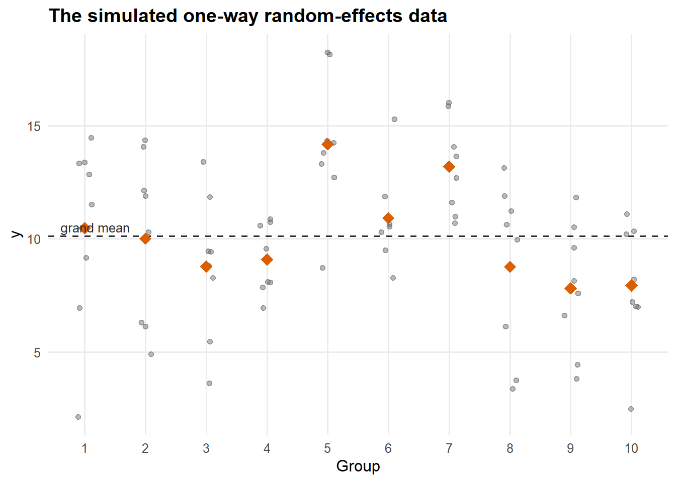
Figure 1: Simulated data. Each light point is an observation; coloured diamonds are group means; the dashed line is the grand mean. The spread of group means reflects \(\sigma_a^2\); the scatter within each column reflects \(\sigma_e^2\).
The entire tutorial is an attempt to recover the three numbers (\(\mu, \sigma_a^2, \sigma_e^2\)) from this picture, using four different logics.
A common notational backbone
The next few sections write the model with matrices, because that is the language MLE and REML are built in. If matrices are not your thing, read the shaded “in plain terms” lines and the figures, and skim past the symbols. Every method also has a simple closed-form answer for our balanced design, and we always show it.
For the methods considered here, it is convenient to express the model in matrix notation. Stacking all observations into the vector \(\mathbf{y}\in\mathbb{R}^N\),
\[ \mathbf{y} \;=\; \mathbf{X}\boldsymbol\beta + \mathbf{Z}\mathbf{a} + \boldsymbol\varepsilon, \] {#eq-matnot}
where \(\mathbf{X} = \mathbf{1}_N\) is the \(N\times 1\) design matrix for the single fixed effect \(\boldsymbol\beta = \mu\) (so \(p = 1\)), \(\mathbf{Z}\) is the \(N\times g\) group-incidence matrix, \(\mathbf{a}\sim\mathcal N(\mathbf 0, \sigma_a^2\mathbf I_g)\), and \(\boldsymbol\varepsilon\sim\mathcal N(\mathbf 0,\sigma_e^2\mathbf I_N)\). Because both the random effects and residual errors are normally distributed, the response vector \(\mathbf{y}\) follows a multivariate normal distribution,
\[ \mathbf{y} \;\sim\; \mathcal{N}\!\big(\mathbf{X}\boldsymbol\beta,\; \mathbf{V}\big) \] {#eq-marginal}
with covariance matrix
\[ \mathbf{V} \;=\; \sigma_a^2\,\mathbf{Z}\mathbf{Z}^\top + \sigma_e^2\,\mathbf{I}_N . \] {#eq-var}
The matrix \(\mathbf{V}\) describes the variance and covariance among all observations. For the balanced one-way random-effects model, \(\mathbf{V}\) is block-diagonal because observations from different groups do not share a random effect and are therefore uncorrelated. Within each group of size \(n\), the covariance has the compound-symmetry form \(\sigma_e^2\mathbf{I}_n + \sigma_a^2\mathbf{J}_n\), where \(\mathbf{J}_n\) is the \(n \times n\) matrix of ones.
\[ \mathbf{V}_{\text{group}} \;=\; \sigma_e^2\,\mathbf{I}_n + \sigma_a^2\,\mathbf{J}_n \;=\; \begin{pmatrix} \sigma_a^2+\sigma_e^2 & \sigma_a^2 & \cdots & \sigma_a^2 \\ \sigma_a^2 & \sigma_a^2+\sigma_e^2 & \cdots & \sigma_a^2 \\ \vdots & \vdots & \ddots & \vdots \\ \sigma_a^2 & \sigma_a^2 & \cdots & \sigma_a^2+\sigma_e^2 \end{pmatrix}. \] {#eq-mat1}
The full covariance matrix is obtained by placing \(g\) identical blocks along the diagonal (\(\mathbf{I}_g \otimes \mathbf{V}_{\text{group}}\)):
\[ \mathbf{V} \;=\; \bigoplus_{i=1}^{g}\mathbf{V}_{\text{group}} \;=\; \begin{pmatrix} \mathbf{V}_{\text{group}} & \mathbf{0} & \cdots & \mathbf{0} \\ \mathbf{0} & \mathbf{V}_{\text{group}} & \cdots & \mathbf{0} \\ \vdots & \vdots & \ddots & \vdots \\ \mathbf{0} & \mathbf{0} & \cdots & \mathbf{V}_{\text{group}} \end{pmatrix} \;=\; \mathbf{I}_g \otimes \mathbf{V}_{\text{group}} . \] {#eq-mat2}
Each observation has variance \(\sigma_a^2+\sigma_e^2\) (the diagonal), and any two observations in the same group share the field or block effect \(\sigma_a^2\) (the off-diagonal). That shared term is exactly the within-group correlation the ICC measures. Keep @eq-marginal in mind: it is the object that MLE and REML optimise.
Finally, the analysis-of-variance decomposition underlies the historical (Method of Moments) estimators and gives clean closed forms we can check everything against. With \(\bar y_{i\cdot}\) the \(i\)-th group mean and \(\bar y_{\cdot\cdot}\) the grand mean,
\[ \underbrace{\sum_{i,j}(y_{ij}-\bar y_{\cdot\cdot})^2}_{SS_{\text{total}}} =\underbrace{n\sum_i (\bar y_{i\cdot}-\bar y_{\cdot\cdot})^2}_{SS_A \;(\text{df}=g-1)} +\underbrace{\sum_{i,j}(y_{ij}-\bar y_{i\cdot})^2}_{SS_E \;(\text{df}=N-g)} . \] {#eq-anova}
ybar    <- mean(y)
ybar_i  <- tapply(y, group, mean)

SS_A <- n * sum((ybar_i - ybar)^2)                       # between groups
SS_E <- sum((y - ybar_i[as.integer(group)])^2)           # within groups
MS_A <- SS_A / (g - 1)                                   # between mean square
MS_E <- SS_E / (N - g)                                   # within  mean square

data.frame(
  Source = c("Between (A)", "Within (E)"),
  df     = c(g - 1, N - g),
  SS     = c(SS_A, SS_E),
  MS     = c(MS_A, MS_E)
)
## Source df SS MS
## 1 Between (A) 9 331.2220 36.802445
## 2 Within (E) 70 640.4952 9.149932We will reuse SS_A, SS_E, MS_A, MS_E repeatedly.
Method of Moments
Philosophy
The Method of Moments (Karl Pearson, 1894) is the oldest general-purpose estimation principle and the most intuitive. A model with \(k\) parameters implies formulas for its first \(k\) theoretical moments as functions of those parameters. The data supply empirical moments. Set the theoretical moments equal to the empirical moments and solve. No optimisation, no distributional likelihood, just a system of equations. It requires the fewest assumptions of any method here (you need the moments to exist, not full normality).
The estimating equations
For a generic parameter vector \(\theta\), let \(\mu_r'(\theta) = \mathbb{E}[Y^r]\) denote the \(r\)-th theoretical raw moment and let \(m_r' = \tfrac1N\sum_i y_i^r\) denote the corresponding sample moment. The method of moments (MoM) estimates the unknown parameters by matching sample moments to their theoretical counterparts. Thus, the MoM estimator \(\hat\theta\) solves
\[ \mu_r'(\hat\theta) \;=\; m_r', \qquad r = 1,2,\dots,k . \] {#eq-mom-general}
Warm-up (a single normal sample). Suppose \(y_i\sim\mathcal N(\mu,\sigma^2)\). The first two theoretical moments are then \(\mu_1'=\mu\) and \(\mu_2'=\mu^2+\sigma^2\). Equating these to the corresponding sample moments yields \(\hat\mu=\bar y\) and \(\hat\sigma^2 = \frac1N\sum_i(y_i-\bar y)^2\), which are simply the sample mean and the sample variance computed using \(N\) in the denominator. Keep that division by \(N\) in mind: it reappears when we discuss MLE and REML.
Moment estimators for the variance components
Our model has a grand mean and two variance components, so we need one additional moment equation beyond the overall mean. In a one-way layout, the natural quantities are the two mean squares, whose expectations are the classical expected mean squares:
\[ \mathbb{E}[MS_E] = \sigma_e^2, \qquad \mathbb{E}[MS_A] = \sigma_e^2 + n\,\sigma_a^2 . \] {#eq-ems}
Sketch of @eq-ems. Within a group, the deviations \(y_{ij}-\bar y_{i\cdot}\) depend only on the \(\varepsilon\) terms, so the within-group sum of squares satisfies \(SS_E/\sigma_e^2\sim\chi^2_{N-g}\), giving \(\mathbb{E}[MS_E]=\sigma_e^2\). For the between-group component, each group mean can be written as \(\bar y_{i\cdot}=\mu+a_i+\bar\varepsilon_{i\cdot}\) with variance \(\sigma_a^2+\sigma_e^2/n\). Expressing the between-group sum of squares on a per-observation scale yields \(\mathbb{E}[MS_A]=\sigma_e^2+n\sigma_a^2\).
Replacing the expectations in @eq-ems by their observed values and solving the \(2\times2\) system gives the ANOVA / Method-of-Moments estimators:
\[ \boxed{\;\hat\mu_{\text{MoM}} = \bar y_{\cdot\cdot},\qquad \hat\sigma^2_{e,\text{MoM}} = MS_E,\qquad \hat\sigma^2_{a,\text{MoM}} = \dfrac{MS_A - MS_E}{n}.\;} \] {#eq-mom-est}
mom <- list(
  mu       = ybar,
  sigma_e2 = MS_E,
  sigma_a2 = (MS_A - MS_E) / n
)
mom$icc <- mom$sigma_a2 / (mom$sigma_a2 + mom$sigma_e2)
unlist(mom)
## mu sigma_e2 sigma_a2 icc
## 10.1173062 9.1499321 3.4565641 0.2741891Visualising the moment match
MoM is “solve a linear system”, so the most honest visual is the system itself: the two observed mean squares and the two parameters that reproduce them through @eq-ems.
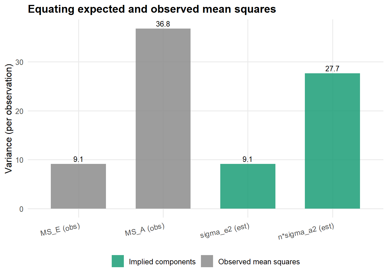
Figure 2: Method of Moments as a balance. The observed mean squares (left) are decomposed into the variance components (right) via \(MS_E=\sigma_e^2\) and \(MS_A=\sigma_e^2+n\sigma_a^2\).
Comparison with the truth
data.frame(
  parameter = c("mu", "sigma_a2", "sigma_e2", "ICC"),
  truth     = c(mu_true, sa2_true, se2_true, icc_true),
  MoM       = c(mom$mu, mom$sigma_a2, mom$sigma_e2, mom$icc)
)
## parameter truth MoM
## 1 mu 10.0000000 10.1173062
## 2 sigma_a2 4.0000000 3.4565641
## 3 sigma_e2 9.0000000 9.1499321
## 4 ICC 0.3076923 0.2741891Uncertainty quantification
For balanced data the relevant sums of squares have exact \(\chi^2\) sampling distributions, which yields an exact confidence interval for the residual variance. Since \(SS_E/\sigma_e^2\sim\chi^2_{N-g}\),
\[ \left[\;\frac{SS_E}{\chi^2_{N-g,\,1-\alpha/2}},\;\; \frac{SS_E}{\chi^2_{N-g,\,\alpha/2}}\;\right] \] {#eq-mom-ci}
is a \(100(1-\alpha)\%\) interval for \(\sigma_e^2\).
alpha <- 0.05
mom_ci_se2 <- SS_E / qchisq(c(1 - alpha/2, alpha/2), df = N - g)

# Standard error of the grand mean under the balanced one-way random-effects
# model. The mean of group means has variance (sigma_a^2 + sigma_e^2/n)/g,
# which is estimated unbiasedly by MS_A/(g*n) since E[MS_A] = n*sigma_a^2 + sigma_e^2.
se_mu_mom <- sqrt(MS_A / (g * n))

setNames(mom_ci_se2, c("lower", "upper"))
## lower upper
## 6.74041 13.13633The between component is harder. \(\hat\sigma_a^2\) is a difference of mean squares, its sampling distribution is not \(\chi^2\), and, notoriously, it can come out negative when \(MS_A < MS_E\). Approximate intervals use Satterthwaite’s effective degrees of freedom,
\[ \nu_{\text{eff}} = \frac{2\,(\hat\sigma_a^2)^2}{\operatorname{Var}(\hat\sigma_a^2)}, \qquad \operatorname{Var}(\hat\sigma_a^2)\approx \frac{2}{n^2}\!\left[\frac{MS_A^2}{g-1}+\frac{MS_E^2}{N-g}\right], \]
after which \(\nu_{\text{eff}}\hat\sigma_a^2/\sigma_a^2 \approx \chi^2_{\nu_{\text{eff}}}\).
var_sa2    <- (2 / n^2) * (MS_A^2 / (g - 1) + MS_E^2 / (N - g))
nu_eff     <- 2 * mom$sigma_a2^2 / var_sa2
mom_ci_sa2 <- nu_eff * mom$sigma_a2 / qchisq(c(1 - alpha/2, alpha/2), df = nu_eff)
c(se_sa2 = sqrt(var_sa2), nu_eff = nu_eff,
  lower = mom_ci_sa2[1], upper = mom_ci_sa2[2])
## se_sa2 nu_eff lower upper
## 2.177205 5.041044 1.350738 20.576662Strengths, weaknesses, assumptions
- Strengths. Distribution-light (needs only that moments exist), closed-form and instantaneous, an excellent starting value for iterative methods, and the conceptual root of GMM. For balanced ANOVA it is also fully efficient.
- Weaknesses. Can produce nonsensical estimates (negative variances); usually less efficient than MLE for non-normal/unbalanced data; uncertainty quantification is awkward and often only approximate; the choice of which moments to match is not unique and affects efficiency.
- Assumptions used here. The first two moments are correctly specified (see @eq-ems) and the design is balanced (so the mean squares are independent and the closed forms are clean).
- Typical applications. Quick variance-component estimates; any setting where a full likelihood is unavailable or undesirable.
Maximum Likelihood Estimation
Philosophy
Fisher’s principle (1922) inverts the usual probabilistic question. Instead of asking “given parameters, how probable is the data?”, it asks “which parameters make the observed data most probable?” The probability of the data, read as a function of the parameters with the data held fixed, is the likelihood. The MLE is its maximiser.
The likelihood and log-likelihood
The likelihood scores a guess: choose values for the parameters \(\boldsymbol\psi = (\boldsymbol\beta,\sigma_a^2,\sigma_e^2)\), and it measures how well those values explain the data you collected, with higher meaning a better fit. Using the marginal model @eq-marginal, that score is the multivariate normal density evaluated at the data:
\[ L(\boldsymbol\psi) = (2\pi)^{-N/2}\,|\mathbf{V}|^{-1/2} \exp\!\Big\{\!-\tfrac12 (\mathbf{y}-\mathbf{X}\boldsymbol\beta)^\top \mathbf{V}^{-1}(\mathbf{y}-\mathbf{X}\boldsymbol\beta)\Big\}. \]
You never work this out by hand; the computer does. Because it multiplies one probability for every observation, the result is a vanishingly small number, so we work on the log scale instead. The log does not change which guess wins, it just keeps the arithmetic stable:
\[ \ell(\boldsymbol\psi) = -\frac{N}{2}\log(2\pi) -\frac12\log|\mathbf{V}| -\frac12(\mathbf{y}-\mathbf{X}\boldsymbol\beta)^\top \mathbf{V}^{-1}(\mathbf{y}-\mathbf{X}\boldsymbol\beta). \] {#eq-loglik}
@eq-loglik is the objective function: the quantity we make as large as possible, pictured in the next section as climbing to the top of a hill.
In plain terms: the score rises when the model’s predictions sit close to the observed values (the last term), but it is penalised for explaining that closeness by simply assuming the data are noisier than they really are (the \(\log|\mathbf{V}|\) term). Balancing those two is what picks out a single best answer.
Profiling out the fixed effect
There is a useful shortcut here. Suppose, for a moment, that we already knew the two variances (and therefore \(\mathbf{V}\)). Then the best grand mean has a tidy formula: the value of \(\boldsymbol\beta\) that maximises @eq-loglik is the generalised least squares (GLS) estimate, found by setting the derivative of the log-likelihood to zero, \(\partial\ell/\partial\boldsymbol\beta=0\):
\[ \hat{\boldsymbol\beta}(\mathbf{V}) = \big(\mathbf{X}^\top\mathbf{V}^{-1}\mathbf{X}\big)^{-1} \mathbf{X}^\top\mathbf{V}^{-1}\mathbf{y}. \] {#eq-gls}
You have likely met the simpler special case. When every observation is independent and has the same variance, so that \(\mathbf{V} = \sigma^2\mathbf{I}\), the formula above collapses to the familiar ordinary least squares (OLS) estimate \(\hat{\boldsymbol\beta} = (\mathbf{X}^\top\mathbf{X})^{-1}\mathbf{X}^\top\mathbf{y}\). GLS is just OLS with the observations re-weighted by \(\mathbf{V}^{-1}\), so that correlated or noisier observations count for less. For our balanced design the two even give the same number, the grand mean \(\bar y_{\cdot\cdot}\); they part ways once the groups become unbalanced.
Because the mean now has a formula written in terms of the variances, we can substitute @eq-gls back into @eq-loglik and be left with a function of the two variances alone, the profile log-likelihood \(\ell_p(\sigma_a^2,\sigma_e^2)\). That is the quantity the computer actually maximises. One practical trick: we search over the logs of the variances, \(\theta_1=\log\sigma_a^2\) and \(\theta_2=\log\sigma_e^2\), so the optimiser can roam freely while the variances themselves stay positive.
X <- matrix(1, N, 1)                     # single fixed effect (intercept = mu)
Z <- model.matrix(~ group - 1)           # N x g group-incidence matrix

make_V <- function(sa2, se2) sa2 * tcrossprod(Z) + se2 * diag(N)

# Negative *profile* log-likelihood (so we can MINIMISE with optim()).
neg_loglik <- function(theta) {
  sa2 <- exp(theta[1]); se2 <- exp(theta[2])
  V   <- make_V(sa2, se2)
  R   <- chol(V)                         # V = R'R, R upper-triangular
  logdetV <- 2 * sum(log(diag(R)))       # stable log-determinant
  Vinv    <- chol2inv(R)
  XtVi    <- crossprod(X, Vinv)
  beta    <- solve(XtVi %*% X, XtVi %*% y)   # GLS estimate, eq. (GLS)
  r       <- y - X %*% beta
  quad    <- as.numeric(crossprod(r, Vinv %*% r))
  0.5 * (N * log(2*pi) + logdetV + quad)     # = -ell_p
}
start <- log(c(var(y) / 2, var(y) / 2)) # crude starting values
fit_ml <- optim(start, neg_loglik, method = "BFGS", hessian = TRUE)
mle <- list(
sigma_a2 = exp(fit_ml$par[1]),
sigma_e2 = exp(fit_ml$par[2]),
loglik = -fit_ml$value
)
# Recover the fixed effect at the optimum via GLS:
Vhat <- make_V(mle$sigma_a2, mle$sigma_e2)
Vinv <- solve(Vhat)
mle$mu <- as.numeric(solve(crossprod(X, Vinv) %*% X, crossprod(X, Vinv) %*% y))
mle$icc <- mle$sigma_a2 / (mle$sigma_a2 + mle$sigma_e2)
unlist(mle[c("mu","sigma_a2","sigma_e2","icc","loglik")])## mu sigma_a2 sigma_e2 icc loglik
## 10.1173062 2.9965344 9.1499324 0.2467001 -208.4972277Closed forms confirm the optimiser
For this balanced design the MLE has a closed form, and comparing it to optim()
reassures us the numerics are right, and exposes the bias that motivates the
next section. The likelihood factorises (because \(\bar y_{\cdot\cdot}\), \(SS_A\) and
\(SS_E\) are mutually independent), giving
\[ \hat\mu_{\text{ML}} = \bar y_{\cdot\cdot},\qquad \hat\sigma^2_{e,\text{ML}} = MS_E,\qquad \hat\sigma^2_{a,\text{ML}} = \frac{1}{n}\!\left(\frac{SS_A}{g} - MS_E\right). \] {#eq-mle-closed}
mle_closed <- c(
  mu       = ybar,
  sigma_e2 = MS_E,
  sigma_a2 = ((SS_A / g) - MS_E) / n     # NOTE the divisor g, not g-1
)
rbind(closed_form = mle_closed,
      optim       = c(mle$mu, mle$sigma_e2, mle$sigma_a2))
## mu sigma_e2 sigma_a2
## closed_form 10.11731 9.149932 2.996534
## optim 10.11731 9.149932 2.996534Compare @eq-mle-closed with the MoM estimator @eq-mom-est. They differ in one place: ML divides the between sum of squares \(SS_A\) by \(g\), the number of groups; MoM (and, as we will see, REML) divides by \(g-1\). That single degree of freedom, the one spent estimating \(\mu\), is the entire story of the next section. Because \(g > g-1\), ML systematically underestimates \(\sigma_a^2\).
Visualising the estimation: the likelihood surface
MLE is hill-climbing on @eq-loglik. Let us draw the hill (over the two variance
components, with \(\mu\) profiled out) and mark where optim() stopped.
sa2_grid <- seq(0.2, 12, length.out = 70)
se2_grid <- seq(5,   14, length.out = 70)
grid <- expand.grid(sa2 = sa2_grid, se2 = se2_grid)
grid$ll <- apply(grid, 1, function(r) -neg_loglik(log(c(r["sa2"], r["se2"]))))
grid$rel <- grid$ll - max(grid$ll)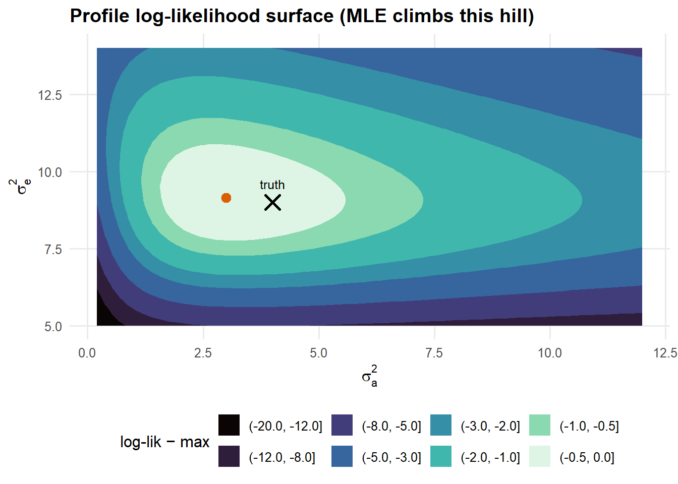
Figure 3: The profile log-likelihood surface over the two variance components, with \(\mu\) concentrated out. The orange dot is the MLE; the black cross is the true \((\sigma_a^2,\sigma_e^2)\). Contours are log-likelihood units below the maximum.
A one-dimensional profile for \(\mu\) makes the curvature-uncertainty link concrete: how sharply the log-likelihood falls away from its peak is the information about \(\mu\).
mu_grid <- seq(mle$mu - 3, mle$mu + 3, length.out = 200)
ll_mu <- sapply(mu_grid, function(m) {
  r <- y - m
  -0.5 * (N * log(2*pi) + as.numeric(determinant(Vhat, TRUE)$modulus) +
          as.numeric(crossprod(r, Vinv %*% r)))
})
prof_mu <- data.frame(mu = mu_grid, rel = ll_mu - max(ll_mu))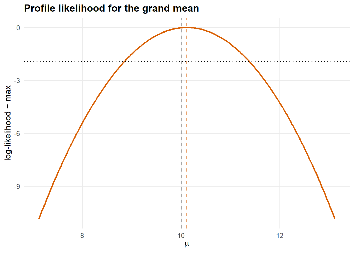
Figure 4: Profile log-likelihood for \(\mu\) (variance components held at their MLEs). Curvature at the peak equals the Fisher information; flatter peaks mean larger standard errors. The horizontal line at \(-1.92\) cuts a 95% likelihood interval.
Comparison with the truth
##   parameter      truth        MoM        MLE
## 1        mu 10.0000000 10.1173062 10.1173062
## 2  sigma_a2  4.0000000  3.4565641  2.9965344
## 3  sigma_e2  9.0000000  9.1499321  9.1499324
## 4       ICC  0.3076923  0.2741891  0.2467001
The MLE of \(\sigma_a^2\) sits below both the truth and the MoM estimate: the expected downward bias.
Uncertainty quantification
How confident should we be in an MLE? The key idea is intuitive: the sharper the peak of the log-likelihood, the more precisely the data pin down the estimate. A narrow, steep peak means only a small range of values fit well, so the standard error is small; a broad, flat peak means many values fit almost equally well, so the estimate is uncertain.
A large-sample result makes this precise. With enough data, an MLE behaves like a draw from a normal distribution centred on the true value, with a spread set by the curvature of that peak:
\[ \hat{\boldsymbol\theta}\;\dot\sim\; \mathcal N\!\big(\boldsymbol\theta,\; \mathcal I(\boldsymbol\theta)^{-1}\big), \qquad \mathcal I(\boldsymbol\theta) = -\,\mathbb{E}\!\left[\frac{\partial^2 \ell}{\partial\boldsymbol\theta\,\partial\boldsymbol\theta^\top}\right]. \]
The matrix \(\mathcal I(\boldsymbol\theta)\), the Fisher information, is just a
measure of that curvature, built from the second derivatives of \(\ell\).
Inverting it turns “how curved” into “how variable,” which gives the variances
and standard errors of the estimates. In practice we read the curvature straight
off the fitted model: the observed information is the Hessian (the matrix of
second derivatives) of \(-\ell\) at the optimum, which optim() already returns.
One last step. Because we maximised on the log-variance scale, the standard errors arrive on that scale too, and the delta method converts them back. If \(\sigma^2 = e^{\theta}\), then \(\widehat{\mathrm{SE}}(\sigma^2) = \sigma^2\,\widehat{\mathrm{SE}}(\theta)\). This is just the chain rule: a small wobble in \(\theta\) shows up as a wobble in \(\sigma^2\) scaled by the derivative \(e^\theta = \sigma^2\).
cov_theta <- solve(fit_ml$hessian)          # covariance of (log sa2, log se2)
se_theta  <- sqrt(diag(cov_theta))

se_sa2 <- mle$sigma_a2 * se_theta[1]        # delta method
se_se2 <- mle$sigma_e2 * se_theta[2]

# Wald 95% CIs are cleanest on the log scale, then back-transformed (keeps them > 0):
ci_sa2 <- exp(fit_ml$par[1] + c(-1, 1) * 1.96 * se_theta[1])
ci_se2 <- exp(fit_ml$par[2] + c(-1, 1) * 1.96 * se_theta[2])

# SE of the GLS mean: Var(mu_hat) = (X' Vinv X)^{-1}
se_mu  <- sqrt(as.numeric(solve(crossprod(X, Vinv) %*% X)))
ci_mu  <- mle$mu + c(-1, 1) * 1.96 * se_mu

data.frame(
  parameter = c("mu", "sigma_a2", "sigma_e2"),
  estimate  = c(mle$mu, mle$sigma_a2, mle$sigma_e2),
  SE        = c(se_mu, se_sa2, se_se2),
  lower95   = c(ci_mu[1], ci_sa2[1], ci_se2[1]),
  upper95   = c(ci_mu[2], ci_sa2[2], ci_se2[2])
)
## parameter estimate SE lower95 upper95
## 1 mu 10.117306 0.6434498 8.8561446 11.37847
## 2 sigma_a2 2.996534 1.8616536 0.8867159 10.12638
## 3 sigma_e2 9.149932 1.5466206 6.5695549 12.74383(The Wald interval for a variance can misbehave near zero; the log-scale construction above avoids negative limits, and a profile-likelihood interval (inverting the curve in @fig-mle-mu-profile) is better still when samples are small.)
Strengths, weaknesses, assumptions
- Strengths. Asymptotically efficient (attains the Cramér–Rao bound), invariant to reparameterisation, a single coherent framework for point estimates and uncertainty, and the basis for likelihood-ratio tests and information criteria (AIC).
- Weaknesses. Variance components are biased in finite samples (the \(\div g\) problem); relies on asymptotics that can be poor with few groups; the full distribution must be specified correctly; the optimisation can be multi-modal or land on a boundary (\(\hat\sigma_a^2 = 0\)).
- Assumptions used here. Correct normal model @eq-marginal; large-sample regularity for the information-based standard errors.
- Typical applications. The default for GLMs, survival models, structural equation models, and as the engine inside almost every modern estimation routine.
Restricted Maximum Likelihood
Philosophy
REML (Patterson & Thompson, 1971) exists to fix one specific flaw: ordinary ML estimates variance components as if the fixed effects were known, when in fact they were estimated from the same data. Estimating \(p\) fixed effects uses up \(p\) degrees of freedom that ML never accounts for, so its variance estimates are biased downward. REML’s remedy is elegant: estimate the variance components from a part of the data that carries no information about the fixed effects, the error contrasts.
The cleanest possible illustration (\(n\) versus \(n-1\))
Take the simplest possible case: a single normal sample \(y_i\sim\mathcal N(\mu,\sigma^2)\). The MLE of the variance, \(\hat\sigma^2_{\text{ML}} = \frac1n\sum(y_i-\bar y)^2\), comes out too small, because we used the same data to estimate \(\bar y\) and then measured the spread around it. The fix is to work with the deviations \(y_i - \bar y\) instead. These \(n-1\) contrasts sum to zero and carry no information about \(\mu\), so building the likelihood from them drops \(\mu\) out of the problem entirely and gives
\[ \hat\sigma^2_{\text{REML}} = \frac{1}{n-1}\sum_i (y_i-\bar y)^2 , \]
the unbiased sample variance Estimating the one mean \(\mu\) cost a single degree of freedom, and REML hands it back. That is the whole idea. Everything below is the same idea written in matrix form.
The restricted likelihood
Rather than analysing the raw responses, REML analyses error contrasts: combinations of the data deliberately built to contain no trace of the fixed effects. Formally, pick any full-rank matrix (A full rank matrix is a matrix where all rows and columns contain zero redundant information, meaning it has the maximum possible number of linearly independent rows or columns for its size) \(\mathbf{K}_{N\times(N-p)}\) with \(\mathbf{K}^\top\mathbf{X}=\mathbf 0\); the transformed data \(\mathbf{K}^\top\mathbf{y}\) are those contrasts. From @eq-marginal,
\[ \mathbf{K}^\top\mathbf{y} \;\sim\; \mathcal N\!\big(\mathbf 0,\; \mathbf{K}^\top\mathbf{V}\mathbf{K}\big), \]
a distribution that does not involve \(\boldsymbol\beta\) at all. Its log-likelihood (which, remarkably, does not depend on which \(\mathbf K\) you pick) is the restricted log-likelihood:
\[ \ell_R(\boldsymbol\theta) = -\frac{N-p}{2}\log(2\pi) -\frac12\log|\mathbf{V}| \;\underbrace{-\frac12\log\big|\mathbf{X}^\top\mathbf{V}^{-1}\mathbf{X}\big|}_{\text{the degrees-of-freedom penalty}} -\frac12(\mathbf{y}-\mathbf{X}\hat{\boldsymbol\beta})^\top \mathbf{V}^{-1}(\mathbf{y}-\mathbf{X}\hat{\boldsymbol\beta}). \] {#eq-reml}
Lined up against the profile ML objective, REML adds exactly one term, \(-\tfrac12\log|\mathbf{X}^\top\mathbf{V}^{-1}\mathbf{X}|\). That term is the price of estimating \(\boldsymbol\beta\): the matrix version of dividing by \(n-1\) instead of \(n\), and it grows larger the more fixed effects you estimate. @eq-reml is the objective function REML optimises.
neg_restricted_loglik <- function(theta) {
  sa2 <- exp(theta[1]); se2 <- exp(theta[2])
  V   <- make_V(sa2, se2)
  R   <- chol(V)
  logdetV <- 2 * sum(log(diag(R)))
  Vinv    <- chol2inv(R)
  XtVi    <- crossprod(X, Vinv)
  XtViX   <- XtVi %*% X
  beta    <- solve(XtViX, XtVi %*% y)
  r       <- y - X %*% beta
  quad    <- as.numeric(crossprod(r, Vinv %*% r))
  p       <- ncol(X)
  logdet_XtViX <- as.numeric(determinant(XtViX, logarithm = TRUE)$modulus)
  # = -ell_R  (the lone extra term vs. neg_loglik is logdet_XtViX)
  0.5 * ((N - p) * log(2*pi) + logdetV + logdet_XtViX + quad)
}
fit_reml <- optim(start, neg_restricted_loglik, method = "BFGS", hessian = TRUE)
reml <- list(
sigma_a2 = exp(fit_reml$par[1]),
sigma_e2 = exp(fit_reml$par[2])
)
Vhat_r <- make_V(reml$sigma_a2, reml$sigma_e2)
Vinv_r <- solve(Vhat_r)
reml$mu <- as.numeric(solve(crossprod(X, Vinv_r) %*% X, crossprod(X, Vinv_r) %*% y))
reml$icc <- reml$sigma_a2 / (reml$sigma_a2 + reml$sigma_e2)
unlist(reml[c("mu","sigma_a2","sigma_e2","icc")])## mu sigma_a2 sigma_e2 icc
## 10.1173062 3.4565333 9.1507465 0.2741696For the balanced one-way model, REML has the closed form
\[ \hat\sigma^2_{e,\text{REML}} = MS_E,\qquad \hat\sigma^2_{a,\text{REML}} = \frac{MS_A - MS_E}{n} = \frac{1}{n}\!\left(\frac{SS_A}{g-1} - MS_E\right), \]
i.e. REML reproduces the ANOVA/MoM estimator exactly: it divides \(SS_A\) by \(g-1\), restoring the degree of freedom that ML dropped.
rbind(
  optim_REML  = c(sigma_a2 = reml$sigma_a2, sigma_e2 = reml$sigma_e2),
  closed_REML = c(sigma_a2 = (MS_A - MS_E)/n, sigma_e2 = MS_E),
  closed_MoM  = c(sigma_a2 = mom$sigma_a2,    sigma_e2 = mom$sigma_e2),
  closed_MLE  = c(sigma_a2 = ((SS_A/g) - MS_E)/n, sigma_e2 = MS_E)
)
## sigma_a2 sigma_e2
## optim_REML 3.456533 9.150746
## closed_REML 3.456564 9.149932
## closed_MoM 3.456564 9.149932
## closed_MLE 2.996534 9.149932# Optional black-box sanity check: lme4 defaults to REML and should match ours.
fm <- lme4::lmer(y ~ 1 + (1 | group), data = dat, REML = TRUE)
vc <- as.data.frame(lme4::VarCorr(fm))
cat("lme4 REML sigma_a2 =", round(vc$vcov[1], 4),
" sigma_e2 =", round(vc$vcov[2], 4), "\n")## lme4 REML sigma_a2 = 3.4566 sigma_e2 = 9.1499cat("ours REML sigma_a2 =", round(reml$sigma_a2, 4),
" sigma_e2 =", round(reml$sigma_e2, 4), "\n")## ours REML sigma_a2 = 3.4565 sigma_e2 = 9.1507Visualising the bias correction
The most instructive REML picture overlays the two profile log-likelihoods for \(\sigma_a^2\), ordinary and restricted, each maximised over \(\sigma_e^2\). The restricted curve’s peak sits to the right of the ML peak: REML pushes the between-group variance estimate upward, undoing the ML bias.
profile_over_se2 <- function(sa2, fn) {
  o <- optimize(function(lse2) fn(c(log(sa2), lse2)),
                lower = log(1e-3), upper = log(1e3))
  -o$objective
}
sa2_seq <- seq(0.05, 12, length.out = 120)
ll_ml   <- sapply(sa2_seq, profile_over_se2, fn = neg_loglik)
ll_reml <- sapply(sa2_seq, profile_over_se2, fn = neg_restricted_loglik)

prof <- rbind(
  data.frame(sigma_a2 = sa2_seq, rel = ll_ml   - max(ll_ml),   method = "MLE"),
  data.frame(sigma_a2 = sa2_seq, rel = ll_reml - max(ll_reml), method = "REML")
)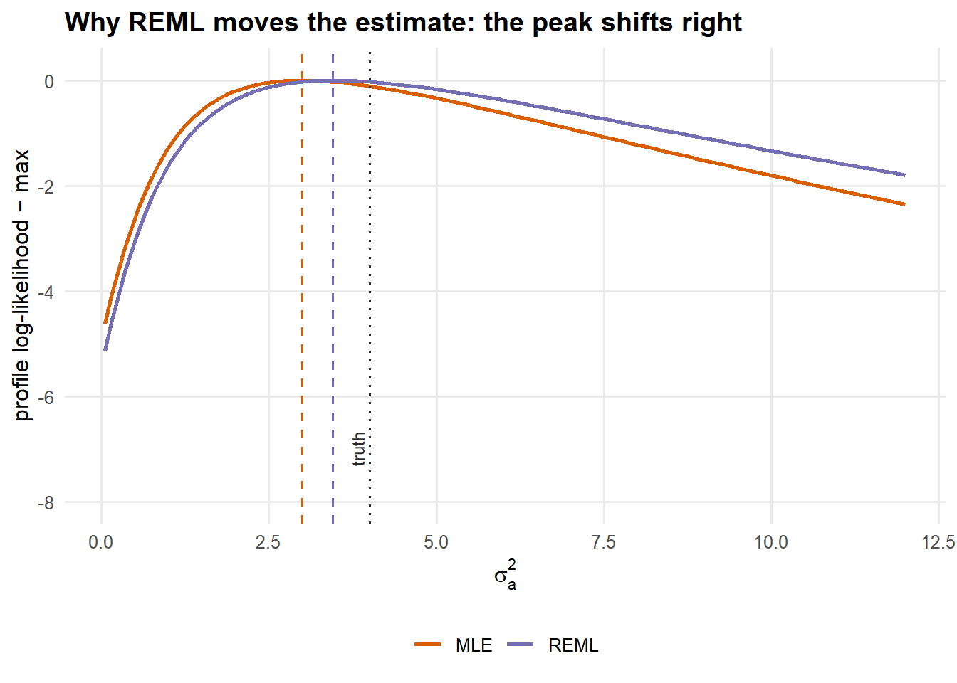
Figure 5: Profile (ordinary) vs. restricted profile log-likelihood for \(\sigma_a^2\), each normalised to peak at zero. REML’s peak is shifted toward the truth, illustrating the bias correction from the extra \(-\tfrac12\log|X^\top V^{-1}X|\) term.
Comparison with the truth
##   parameter      truth        MLE       REML
## 1        mu 10.0000000 10.1173062 10.1173062
## 2  sigma_a2  4.0000000  2.9965344  3.4565333
## 3  sigma_e2  9.0000000  9.1499324  9.1507465
## 4       ICC  0.3076923  0.2467001  0.2741696
Uncertainty quantification
Inference proceeds exactly as for ML, but using the Hessian of @eq-reml. The resulting standard errors for variance components are generally better calibrated in small samples because the objective already accounts for fixed- effect estimation. The standard error of \(\hat\mu\) still comes from the GLS formula \(\operatorname{Var}(\hat\mu)=(\mathbf X^\top\mathbf V^{-1}\mathbf X)^{-1}\), now evaluated at the REML \(\mathbf V\).
cov_theta_r <- solve(fit_reml$hessian)
se_theta_r  <- sqrt(diag(cov_theta_r))
se_sa2_r <- reml$sigma_a2 * se_theta_r[1]
se_se2_r <- reml$sigma_e2 * se_theta_r[2]
se_mu_r  <- sqrt(as.numeric(solve(crossprod(X, Vinv_r) %*% X)))

data.frame(
  parameter = c("mu", "sigma_a2", "sigma_e2"),
  estimate  = c(reml$mu, reml$sigma_a2, reml$sigma_e2),
  SE        = c(se_mu_r, se_sa2_r, se_se2_r),
  lower95   = c(reml$mu - 1.96*se_mu_r, exp(fit_reml$par[1] - 1.96*se_theta_r[1]),
                exp(fit_reml$par[2] - 1.96*se_theta_r[2])),
  upper95   = c(reml$mu + 1.96*se_mu_r, exp(fit_reml$par[1] + 1.96*se_theta_r[1]),
                exp(fit_reml$par[2] + 1.96*se_theta_r[2]))
)
## parameter estimate SE lower95 upper95
## 1 mu 10.117306 0.6782608 8.787915 11.44670
## 2 sigma_a2 3.456533 2.1772520 1.005689 11.88004
## 3 sigma_e2 9.150746 1.5468265 6.570043 12.74515Strengths, weaknesses, assumptions
- Strengths. (Approximately, and for balanced data exactly) unbiased variance components; the de-facto standard for linear mixed models; better small-sample calibration than ML.
- Weaknesses. The restricted likelihood depends on the fixed-effects design, so you cannot use REML likelihoods to compare models with different fixed effects (likelihood-ratio tests and AIC across different \(\mathbf{X}\) are invalid under REML, refit with ML for those). It still assumes normality, and still gives only point + asymptotic-SE inference.
- Assumptions used here. Same normal model @eq-marginal; the contrasts \(\mathbf K^\top\mathbf y\) are exactly normal.
- Typical applications. Variance-component and heritability estimation, animal/plant breeding, multilevel and longitudinal models, anywhere unbiased variance estimates matter and the fixed-effects structure is fixed.
Bayesian Estimation
Philosophy
The methods so far treated the parameters \(\mu,\sigma_a^2,\sigma_e^2\) as fixed but unknown numbers, and asked which values the data point to. The Bayesian view starts somewhere different: it treats every unknown (the parameters, and even the unobserved group effects \(a_i\)) as a random variable described by a probability distribution. This does not claim the parameter is physically random; the distribution simply encodes how sure we are about its value.
Estimation then becomes learning from data. We begin with a prior distribution \(p(\boldsymbol\theta)\), our beliefs before seeing the data. The data enter through the likelihood \(p(\mathbf y\mid\boldsymbol\theta)\), the very same density we maximised for MLE. Bayes’ theorem combines the two into a posterior distribution \(p(\boldsymbol\theta\mid\mathbf y)\), our updated beliefs after seeing the data:
\[ p(\boldsymbol\theta\mid\mathbf y) = \frac{p(\mathbf y\mid\boldsymbol\theta)\,p(\boldsymbol\theta)}{p(\mathbf y)} \;\propto\; \underbrace{p(\mathbf y\mid\boldsymbol\theta)}_{\text{likelihood}}\; \underbrace{p(\boldsymbol\theta)}_{\text{prior}} . \] {#eq-bayes}
In words: the posterior is proportional to the likelihood times the prior. The answer is not a single number but a whole distribution. We summarise it by its centre (the posterior mean or median, which serves as a point estimate) and its spread (a 95% credible interval, the range that holds the parameter with 95% posterior probability). That phrase is worth pausing on: a credible interval means exactly what people usually, and incorrectly, believe a confidence interval means.
The one awkward piece is the denominator \(p(\mathbf y)\), a normalising constant that is almost always impossible to compute directly. The idea that makes modern Bayesian analysis practical is to sidestep it entirely by drawing samples from the posterior rather than writing it down in closed form.
Model, priors, and conjugacy
We write the model in its hierarchical form, keeping the group effects \(a_i\) in as unknowns to be estimated alongside everything else:
\[ \begin{aligned} y_{ij}\mid \mu, a_i, \sigma_e^2 &\sim \mathcal N(\mu + a_i,\ \sigma_e^2), \\ a_i\mid\sigma_a^2 &\sim \mathcal N(0,\ \sigma_a^2), \end{aligned} \qquad\text{with priors}\qquad \begin{aligned} \mu &\sim \mathcal N(\mu_0,\ \gamma_0^2), \\ \sigma_e^2 &\sim \text{Inv-Gamma}(a_e, b_e), \\ \sigma_a^2 &\sim \text{Inv-Gamma}(a_a, b_a). \end{aligned} \]
These particular prior families are not arbitrary; they are chosen to make the updating clean. A prior is conjugate to the likelihood when the resulting posterior belongs to the same family as the prior. Conjugacy is a convenience rather than a requirement, but a powerful one: it means each update has an exact, closed-form answer, so we can sample from it directly with no approximation. Two classic conjugate pairs appear here:
- A Normal prior on a mean, combined with Normal data, yields a Normal posterior. That is why the grand mean \(\mu\) receives a Normal prior.
- An Inverse-Gamma prior on a variance, combined with Normal data, yields an Inverse-Gamma posterior. The Inverse-Gamma also lives only on the positive numbers, which is exactly what a variance requires. That is why \(\sigma_e^2\) and \(\sigma_a^2\) receive Inverse-Gamma priors.
We use weakly informative defaults that let the data dominate: a near-flat \(\mathcal N(0,10^6)\) on \(\mu\) and \(\text{Inv-Gamma}(0.001,0.001)\) on each variance. (More on this choice, and its known fragility for variance components, below.)
Deriving the Gibbs sampler
We still cannot write the full posterior as one tidy distribution. But thanks to conjugacy we can write down, for each unknown, its full conditional: the distribution of that one parameter given the data and the current values of all the others. Each full conditional turns out to be a familiar, easy-to-sample family.
The Gibbs sampler exploits this. Starting from any reasonable values, it visits the unknowns one at a time, replacing each with a fresh draw from its full conditional while holding the others fixed, and then repeats this cycle thousands of times. Remarkably, the values it visits settle into genuine draws from the joint posterior, and the intractable constant \(p(\mathbf y)\) never has to be computed. The four full conditionals, with \(\bar y_{i\cdot}\) the \(i\)-th group mean, are as follows.
Group effects (a precision-weighted shrinkage toward zero):
\[ a_i \mid \cdots \;\sim\; \mathcal N\!\left( \frac{(n/\sigma_e^2)(\bar y_{i\cdot}-\mu)}{n/\sigma_e^2 + 1/\sigma_a^2}, \;\; \frac{1}{n/\sigma_e^2 + 1/\sigma_a^2} \right). \]
In plain terms: each group’s effect is estimated as a compromise between what that group’s own data say (\(\bar y_{i\cdot}-\mu\)) and zero, weighted by how much data the group has against how variable groups are. Groups with little data, or data that look like everyone else’s, get pulled harder toward zero. This automatic shrinkage (the same idea as a BLUP in breeding work) is one of the most useful features of hierarchical models.
Grand mean (a Normal prior updated by Normal data gives a Normal posterior):
\[ \mu \mid \cdots \;\sim\; \mathcal N\!\left( \frac{\mu_0/\gamma_0^2 + \big(\sum_{i,j}(y_{ij}-a_i)\big)/\sigma_e^2} {1/\gamma_0^2 + N/\sigma_e^2}, \;\; \frac{1}{1/\gamma_0^2 + N/\sigma_e^2} \right). \]
In plain terms: the updated mean is a weighted average of the prior guess \(\mu_0\) and the data average (after the group effects are removed), each weighted by its precision, which is one over its variance, that is, how informative it is. A near-flat prior carries almost no precision, so the data effectively decide \(\mu\).
Residual variance (Inverse-Gamma prior, Normal data, Inverse-Gamma posterior):
\[ \sigma_e^2 \mid \cdots \;\sim\; \text{Inv-Gamma}\!\left(a_e + \tfrac{N}{2},\;\; b_e + \tfrac12\sum_{i,j}(y_{ij}-\mu-a_i)^2\right). \]
In plain terms: the posterior keeps the Inverse-Gamma shape, with its second parameter increased by the leftover within-group variation \(\sum(y_{ij}-\mu-a_i)^2\). More residual scatter pushes \(\sigma_e^2\) higher, exactly as intuition demands.
Between-group variance (the same Inverse-Gamma conjugacy):
\[ \sigma_a^2 \mid \cdots \;\sim\; \text{Inv-Gamma}\!\left(a_a + \tfrac{g}{2},\;\; b_a + \tfrac12\sum_{i} a_i^2\right). \]
In plain terms: identical in spirit, now driven by how spread out the estimated group effects \(a_i\) are. Widely differing groups push \(\sigma_a^2\) up; near-identical groups pull it toward zero.
# Sample from Inv-Gamma(shape, rate) as 1 / Gamma(shape, rate).
gibbs_one_way <- function(y, group, n_iter = 12000, burn = 2000,
                          mu0 = 0, g0_2 = 1e6,
                          a_e = 1e-3, b_e = 1e-3,
                          a_a = 1e-3, b_a = 1e-3, seed = 1) {
  set.seed(seed)
  group  <- factor(group); lev <- levels(group)
  g <- length(lev); N <- length(y); gidx <- as.integer(group)
  n_i    <- as.numeric(table(group))
  ybar_i <- as.numeric(tapply(y, group, mean))

  draws <- matrix(NA_real_, n_iter, 3,
                  dimnames = list(NULL, c("mu", "sigma_a2", "sigma_e2")))

  mu <- mean(y); se2 <- var(y) / 2; sa2 <- var(y) / 2; a <- numeric(g)  # init

  for (t in seq_len(n_iter)) {
    ## 1) group effects a_i
    prec_a <- n_i / se2 + 1 / sa2
    a <- rnorm(g, mean = (n_i / se2) * (ybar_i - mu) / prec_a,
                  sd   = sqrt(1 / prec_a))
    ## 2) grand mean mu
    prec_mu <- 1 / g0_2 + N / se2
    s_resid <- sum(n_i * (ybar_i - a))            # = sum_ij (y_ij - a_i)
    mu <- rnorm(1, mean = (mu0 / g0_2 + s_resid / se2) / prec_mu,
                   sd   = sqrt(1 / prec_mu))
    ## 3) residual variance sigma_e^2
    rss <- sum((y - mu - a[gidx])^2)
    se2 <- 1 / rgamma(1, shape = a_e + N / 2, rate = b_e + rss / 2)
    ## 4) between variance sigma_a^2
    sa2 <- 1 / rgamma(1, shape = a_a + g / 2, rate = b_a + sum(a^2) / 2)

    draws[t, ] <- c(mu, sa2, se2)
  }
  draws[(burn + 1):n_iter, , drop = FALSE]
}

post <- gibbs_one_way(y, group)
post_icc <- post[, "sigma_a2"] / (post[, "sigma_a2"] + post[, "sigma_e2"])
nrow(post)   # retained posterior draws
## [1] 10000Did the sampler work? Trace plots
Before trusting any summary we check that the chains mixed and reached a stationary regime (no trend, good exploration).
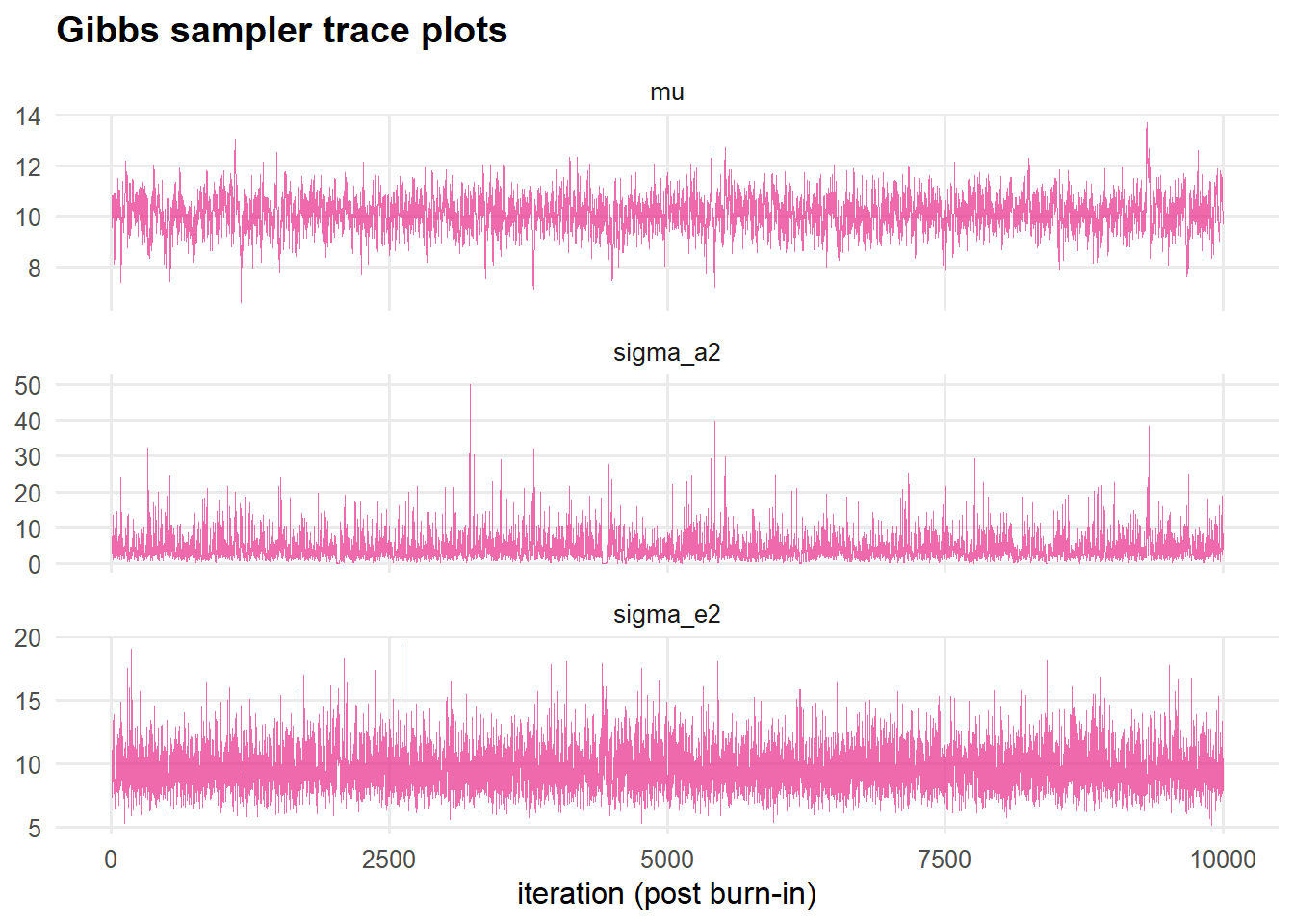
Figure 6: Trace plots of the retained draws. Stationary, well-mixed ‘fuzzy caterpillars’ indicate the sampler is exploring the posterior rather than drifting.
Posterior distributions and credible intervals
The posterior is the inference. We summarise each margin by its mean and a 95% equal-tailed credible interval, the central interval containing 95% of the posterior probability.
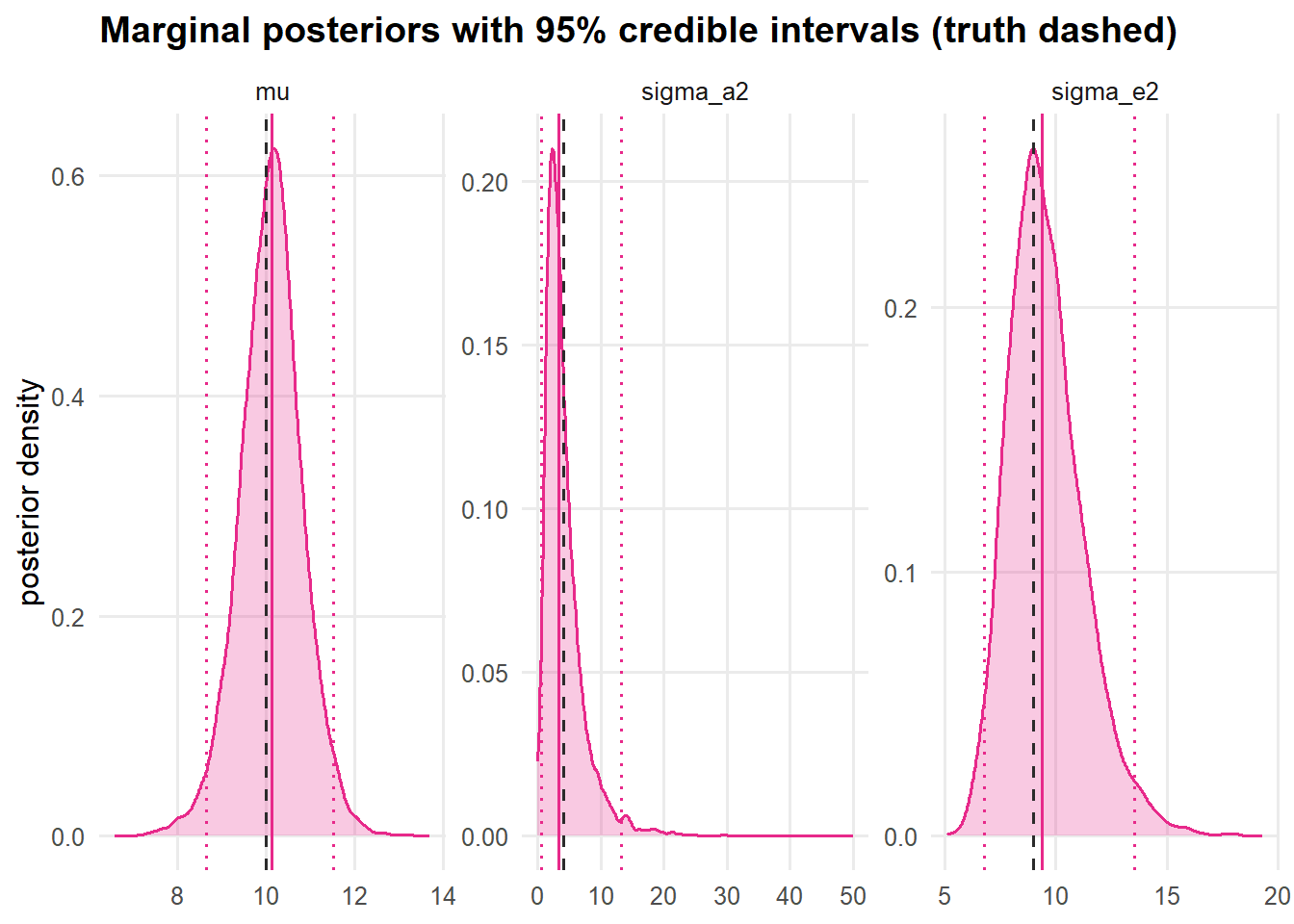
Figure 7: Marginal posteriors. Solid line = posterior mean; shaded band = 95% credible interval; dashed line = the true value. The posteriors comfortably cover the truth.
bayes_summary <- function(x)
  c(mean = mean(x), median = median(x),
    lower95 = unname(quantile(x, 0.025)), upper95 = unname(quantile(x, 0.975)))

bayes <- rbind(
  mu       = bayes_summary(post[, "mu"]),
  sigma_a2 = bayes_summary(post[, "sigma_a2"]),
  sigma_e2 = bayes_summary(post[, "sigma_e2"]),
  ICC      = bayes_summary(post_icc)
)
round(bayes, 3)
## mean median lower95 upper95
## mu 10.111 10.125 8.650 11.525
## sigma_a2 4.137 3.282 0.607 13.201
## sigma_e2 9.575 9.368 6.802 13.531
## ICC 0.277 0.261 0.051 0.594Notice the ICC row: with the full posterior in hand, uncertainty for any function of the parameters comes for free: we just transform each draw, with no delta-method approximation. This is a genuine practical advantage of the Bayesian machinery.
How a prior updates into a posterior
The defining Bayesian act is updating. To see it without distraction, give \(\mu\) a deliberately informative (and deliberately wrong) prior centred at 8, then watch the data drag the posterior toward the truth near 10.
post_inform <- gibbs_one_way(y, group, mu0 = 8, g0_2 = 1, seed = 7)  # tight wrong prior
post_vague  <- post                                                  # the main, vague-prior run

xg <- seq(6, 12, length.out = 400)
prior_dens <- dnorm(xg, mean = 8, sd = 1)                            # the informative prior

upd <- rbind(
  data.frame(mu = xg, dens = prior_dens, kind = "Prior  N(8, 1)"),
  data.frame(mu = density(post_inform[, "mu"], from = 6, to = 12, n = 400)$x,
             dens = density(post_inform[, "mu"], from = 6, to = 12, n = 400)$y,
             kind = "Posterior (informative prior)"),
  data.frame(mu = density(post_vague[, "mu"], from = 6, to = 12, n = 400)$x,
             dens = density(post_vague[, "mu"], from = 6, to = 12, n = 400)$y,
             kind = "Posterior (vague prior) ~ likelihood")
)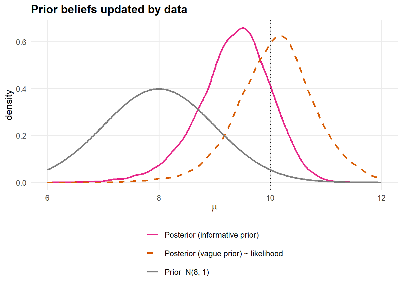
Figure 8: Belief updating for \(\mu\). A confident-but-wrong prior centred at 8 (grey) is pulled by the data toward \(\approx 10\) (pink). With a vague prior, the posterior essentially equals the likelihood (orange dashed). The data dominate the wrong prior.
A word on variance priors (and why it matters)
The \(\text{Inv-Gamma}(\epsilon,\epsilon)\) prior is conjugate and convenient, but Gelman (2006) showed it can be surprisingly informative for hierarchical variances: when the number of groups is small or the true variance is near zero, the posterior can be sensitive to \(\epsilon\). A robust modern default is a half-Normal or half-Cauchy prior on the standard deviation \(\sigma_a\). We can probe sensitivity here by re-running with a different inverse-gamma scale:
post_alt <- gibbs_one_way(y, group, a_a = 2, b_a = 4, seed = 3)  # IG(2, 4): mean ~ 4
rbind(
  `IG(0.001,0.001)` = c(sigma_a2_mean = mean(post[, "sigma_a2"]),
                        sigma_a2_med  = median(post[, "sigma_a2"])),
  `IG(2,4)`         = c(sigma_a2_mean = mean(post_alt[, "sigma_a2"]),
                        sigma_a2_med  = median(post_alt[, "sigma_a2"]))
)
## sigma_a2_mean sigma_a2_med
## IG(0.001,0.001) 4.137276 3.282043
## IG(2,4) 3.191633 2.748499With 10 groups the two priors broadly agree, but the gap would widen with fewer groups, which is why you should always report prior sensitivity for variance components.
Strengths, weaknesses, assumptions
- Strengths. A full distribution rather than a point; exact (simulation-based) uncertainty for any function of the parameters; principled incorporation of external knowledge; automatic, interpretable shrinkage of group effects; valid in small samples without asymptotics; coherent propagation of uncertainty through to predictions.
- Weaknesses. Requires priors (a feature and a responsibility); results can be prior-sensitive for variances; computationally heavier; needs convergence diagnostics; the interpretation differs fundamentally from frequentist output.
- Assumptions used here. The likelihood @eq-marginal and the specified priors; for the Gibbs sampler, conditional conjugacy; for valid summaries, convergence of the chain.
- Typical applications. Hierarchical/multilevel modelling, small-sample or sparse-data problems, evidence synthesis, decision analysis, and anywhere full uncertainty propagation or prior information is valuable.
Synthesis and comparison
We applied four estimation logics to one dataset whose truth we know. Now we put them side by side.
Point estimates
##   parameter  Truth    MoM    MLE   REML  Bayes
## 1        mu 10.000 10.117 10.117 10.117 10.111
## 2  sigma_a2  4.000  3.457  2.997  3.457  4.137
## 3  sigma_e2  9.000  9.150  9.150  9.151  9.575
## 4       ICC  0.308  0.274  0.247  0.274  0.277
The pattern is exactly the theory: MoM = REML (both divide \(SS_A\) by \(g-1\)); MLE sits below them on \(\sigma_a^2\) (divides by \(g\), the finite-sample downward bias); the Bayesian posterior mean lands near REML but is pulled a touch higher by the prior and by averaging over a right-skewed posterior. All four agree closely on \(\mu\) and \(\sigma_e^2\), where there is no degrees-of- freedom subtlety.
Variance estimates and uncertainty, side by side
## Warning: The `fatten` argument of `geom_pointrange()` is deprecated as of ggplot2 4.0.0.
## ℹ Please use the `size` aesthetic instead.
## This warning is displayed once per session.
## Call `lifecycle::last_lifecycle_warnings()` to see where this warning was
## generated.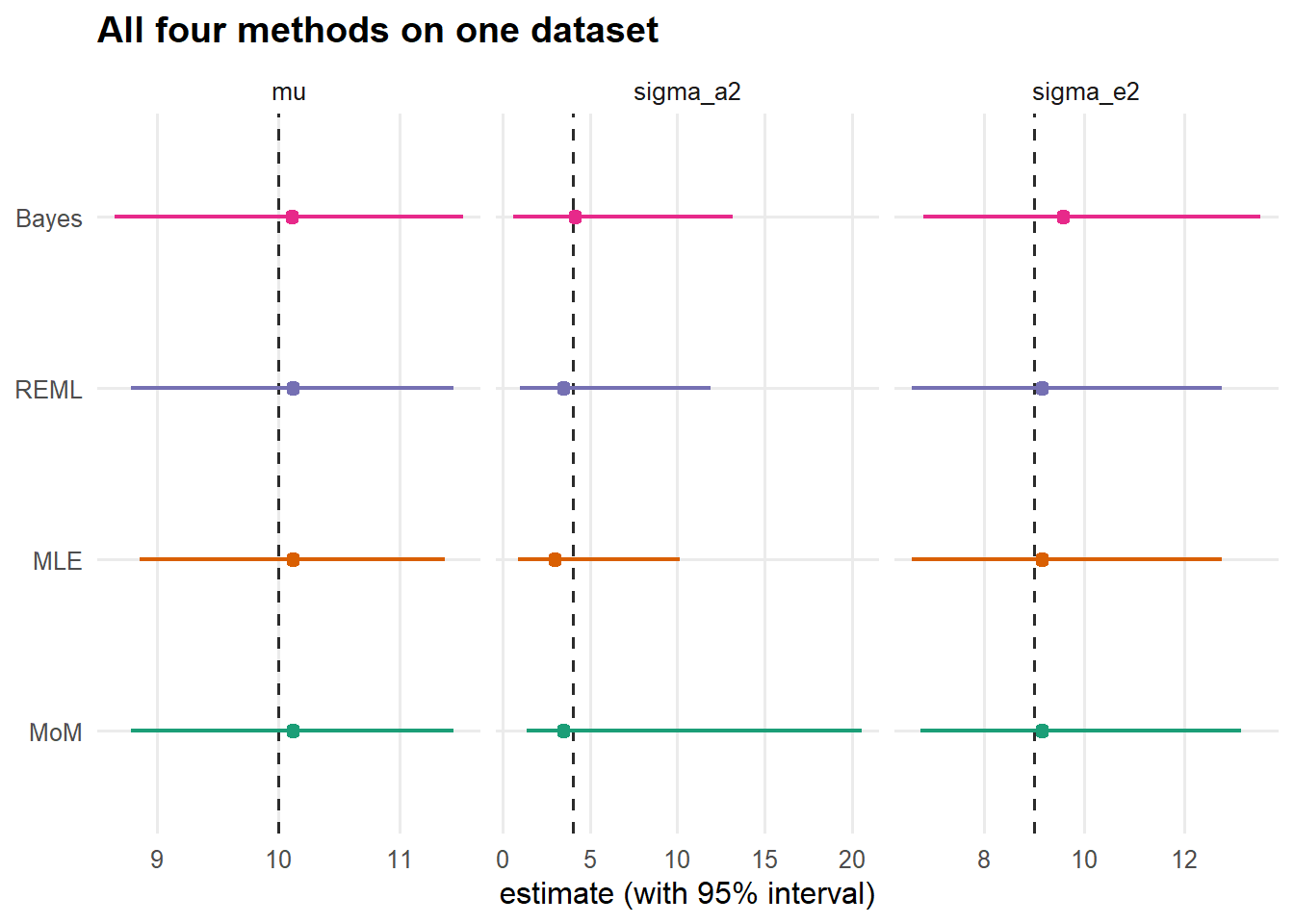
Figure 9: Point estimates with uncertainty for each parameter and method. Bars are 95% intervals (Wald/χ² for the frequentist methods, credible for Bayes). Dashed line = truth. The methods agree on \(\mu\) and \(\sigma_e^2\) and diverge, as theory predicts, on the between-group variance \(\sigma_a^2\).
A structured comparison
| Aspect | MoM | MLE | REML | Bayes |
|---|---|---|---|---|
| Point estimate of variance components | MS_A, MS_E solved | Maximise ℓ | Maximise ℓ_R | Posterior mean/median |
| Treatment of uncertainty | Approx / χ²-based | Fisher information | Information from ℓ_R | Full posterior |
| Interval interpretation | Confidence | Confidence | Confidence | Credible |
| Finite-sample bias (variance comps.) | Unbiased (balanced) | Downward biased | Reduced / unbiased (balanced) | Depends on prior |
| Distributional assumption | Moments only | Full likelihood | Full likelihood | Likelihood + prior |
| Computational cost | Trivial (closed form) | Low to moderate | Low to moderate | High (MCMC) |
| Compares models w/ different fixed effects? | N/A | Yes (LRT, AIC) | No (refit with ML) | Yes (Bayes factors / IC) |
| Uncertainty for functions of params (e.g. ICC) | Awkward (delta/Satterthwaite) | Delta method | Delta method | Exact from draws |
Frequentist versus Bayesian interpretation
The single most important distinction is what an interval means.
- A 95% confidence interval (MoM, MLE, REML) is a statement about the procedure: across hypothetical repetitions of the experiment, 95% of the intervals so constructed would contain the fixed, unknown \(\theta\). The interval is random; \(\theta\) is fixed. You may not say “there is a 95% probability \(\theta\) is in this interval.”
- A 95% credible interval (Bayes) is a statement about the parameter: given this data, prior, and model, there is a 95% posterior probability that \(\theta\) lies in the interval. \(\theta\) is random; the interval is fixed once data are observed. This is the statement people wish a confidence interval made, and only the Bayesian framework licenses it.
These often look numerically similar (compare the bars in @fig-forest), but they answer different questions, and they can diverge sharply with small samples, strong priors, or near a boundary like \(\sigma_a^2 = 0\).
Which method, when?
- Method of Moments: when you need a fast answer, a starting value for an iterative fit, or you are unwilling to assume a full distribution (the GMM spirit). Excellent for balanced designs.
- Maximum Likelihood: your default for point estimation and testing, especially when you must compare models with different fixed effects (LRTs, AIC) or when the sample is large enough that finite-sample variance bias is negligible.
- REML: the standard for variance components and mixed models whenever unbiased variance estimates matter and the fixed-effects structure is settled; prefer it over ML for the final variance estimates, but switch back to ML to compare fixed-effects specifications.
- Bayesian: when the sample is small or the model deeply hierarchical, when you have genuine prior information, when you need exact uncertainty for derived quantities (predictions, ICCs, ratios), or when full uncertainty propagation into a downstream decision is the goal.
The takeaway
All four methods answer the same question, “what parameter values fit this data?”, and they differ only in how they ask it. On our balanced design that difference collapsed to a single arithmetic choice: dividing the between-group sum of squares by \(g\) (ML) or by \(g-1\) (MoM, REML, and effectively the Bayesian posterior). They agreed where the problem is easy, on \(\mu\) and \(\sigma_e^2\), and disagreed exactly where a degree of freedom and the prior have something to say, on \(\sigma_a^2\). Knowing why they disagree is what lets you read any of these outputs with confidence.
Vini Garnica
Assistant Professor
Quantitative plant pathologist developing data-driven tools for disease prediction and crop management.