Mapping and Sampling Wheat Fields in North Carolina using R

Introduction

In this post, I’ll walk you through a workflow for mapping and sampling agricultural fields in the U.S., using wheat in North Carolina as an example.

Randomly selecting coordinates of agricultural fields is important when testing a model. It helps ensure that the sample accurately represents the larger area, making it possible to confirm that the model’s predictions are reliable.

For instance, imagine you’ve developed a model to predict crop yield in a particular region. Since meteorological conditions significantly affect crop yield, it’s logical to include these factors as predictors in your model. Using your expertise, you create meteorological predictors and estimate their effects using a statistical model. However, an important question remains: how well do your meteorological data match the historical patterns in the region? You can assess this by sampling random points in the entire region and comparing the distribution of these variables.

Of course, random sampling across the entire target area (here, the state) will also yield coordinates for locations that aren’t agricultural, such as forests, urban areas, and water bodies. Since agricultural production is often clustered, a more efficient approach is to obtain coordinates only from fields planted with the crop you’re modeling. This targeted sampling ensures your model is both accurate and relevant to the specific agricultural landscape.

In this tutorial, we will leverage various packages like CropScapeR, terra, and sf to handle geospatial data. I’ll show you how to extract and process specific crop data, randomly sample field locations in the target region, and create geocoordinates to be used in the future for model validation. The final output will be a dataset that includes wheat field coordinates ready for further analysis or fieldwork planning.

Packages Setup

Let’s start by loading the necessary packages. If you don’t have them installed, you can install them using install.packages() or the pacman package.

pacman::p_load(data.table,   # Data manipulation
               tidyverse,    # Data science tools (e.g., dplyr, ggplot2)
               CropScapeR,   # Access to Cropland Data Layer (CDL)
               sf,           # Handling spatial vector data (points, lines, polygons)
               tigris,       # Access to U.S. Census geographic data
               terra)        # Manipulation and analysis of raster data

Helper functions

Here’s a helper function that converts a raster into a data frame, making it easier to manipulate and visualize.

rasterdf = function(x, aggregate = 1) {
  resampleFactor = aggregate        
  inputRaster = x    
  inCols = ncol(inputRaster)
  inRows = nrow(inputRaster)
  resampledRaster = rast(ncol=(inCols / resampleFactor), 
                         nrow=(inRows / resampleFactor),
                         crs = crs(inputRaster))
  ext(resampledRaster) = ext(inputRaster)
  y = resample(inputRaster,resampledRaster,method='near')
  coords = xyFromCell(y, seq_len(ncell(y)))
  dat = stack(values(y, dataframe = TRUE))
  names(dat) = c('value', 'variable')
  dat = cbind(coords, dat)
  dat
}

### obs: This function was found online and I don't remember the source

GetCDLData: Download the CDL data as raster data

Next, we’ll download the CDL data for 2022 and load it as a raster object.

The Cropland Data Layer (CDL) is a detailed raster dataset that categorizes agricultural land use across the United States. It provides yearly information on where specific crops, such as corn, soybeans, and wheat, are grown. These maps are created by the United States Department of Agriculture (USDA), which gathers extensive field-level data directly from farmers. This data is then used to train machine learning models that predict the spatial distribution of different crops using satellite imagery. While the CDL datasets are available for visualization on the CropScape online platform (https://nassgeodata.gmu.edu/CropScape/), they can also be accessed directly in R using the CropScapeR package.

cdl = GetCDLData(aoi = '37', year = 2022, type = 'f')
cdl = terra::rast(cdl)

There are three main parameters in this function:

  • aoi: Area of Interest (AOI).
  • year: Year of the data to request.
  • type: Type of AOI.

In this example, we use a state (defined by a 2-digit state FIPS code) as the AOI type, indicated by type = f. North Carolina’s FIPS code is 37. The downloaded data is stored as a RasterLayer object. Note that the CDL data uses the Albers equal-area conic projection. For more information on AOI types, check this out.

cdl
## class       : SpatRaster 
## dimensions  : 11455, 25976, 1  (nrow, ncol, nlyr)
## resolution  : 30, 30  (x, y)
## extent      : 1054155, 1833435, 1345215, 1688865  (xmin, xmax, ymin, ymax)
## coord. ref. : +proj=aea +lat_0=23 +lon_0=-96 +lat_1=29.5 +lat_2=45.5 +x_0=0 +y_0=0 +datum=NAD83 +units=m +no_defs 
## source      : CDL_2022_37.tif 
## color table : 1 
## name        : Layer_1

The downloaded data is a RasterLayer object. CDL data uses the Albers equal-area conic projection, which can be checked as follows:

terra::crs(cdl) 
## [1] "PROJCRS[\"unknown\",\n    BASEGEOGCRS[\"unknown\",\n        DATUM[\"North American Datum 1983\",\n            ELLIPSOID[\"GRS 1980\",6378137,298.257222101,\n                LENGTHUNIT[\"metre\",1]],\n            ID[\"EPSG\",6269]],\n        PRIMEM[\"Greenwich\",0,\n            ANGLEUNIT[\"degree\",0.0174532925199433],\n            ID[\"EPSG\",8901]]],\n    CONVERSION[\"unknown\",\n        METHOD[\"Albers Equal Area\",\n            ID[\"EPSG\",9822]],\n        PARAMETER[\"Latitude of false origin\",23,\n            ANGLEUNIT[\"degree\",0.0174532925199433],\n            ID[\"EPSG\",8821]],\n        PARAMETER[\"Longitude of false origin\",-96,\n            ANGLEUNIT[\"degree\",0.0174532925199433],\n            ID[\"EPSG\",8822]],\n        PARAMETER[\"Latitude of 1st standard parallel\",29.5,\n            ANGLEUNIT[\"degree\",0.0174532925199433],\n            ID[\"EPSG\",8823]],\n        PARAMETER[\"Latitude of 2nd standard parallel\",45.5,\n            ANGLEUNIT[\"degree\",0.0174532925199433],\n            ID[\"EPSG\",8824]],\n        PARAMETER[\"Easting at false origin\",0,\n            LENGTHUNIT[\"metre\",1],\n            ID[\"EPSG\",8826]],\n        PARAMETER[\"Northing at false origin\",0,\n            LENGTHUNIT[\"metre\",1],\n            ID[\"EPSG\",8827]]],\n    CS[Cartesian,2],\n        AXIS[\"(E)\",east,\n            ORDER[1],\n            LENGTHUNIT[\"metre\",1,\n                ID[\"EPSG\",9001]]],\n        AXIS[\"(N)\",north,\n            ORDER[2],\n            LENGTHUNIT[\"metre\",1,\n                ID[\"EPSG\",9001]]]]"

Downloading county and state data

Let’s download the 2022 CDL data for Lenoir, Duplin, and Wayne Counties in North Carolina and visualize the selected area.

NC_county = tigris::counties(state = "NC", cb = TRUE) %>% 
  st_as_sf() 
##   |                                                                              |                                                                      |   0%  |                                                                              |                                                                      |   1%  |                                                                              |=                                                                     |   1%  |                                                                              |=                                                                     |   2%  |                                                                              |==                                                                    |   2%  |                                                                              |==                                                                    |   3%  |                                                                              |===                                                                   |   4%  |                                                                              |===                                                                   |   5%  |                                                                              |====                                                                  |   5%  |                                                                              |====                                                                  |   6%  |                                                                              |=====                                                                 |   7%  |                                                                              |=====                                                                 |   8%  |                                                                              |======                                                                |   8%  |                                                                              |======                                                                |   9%  |                                                                              |=======                                                               |   9%  |                                                                              |=======                                                               |  10%  |                                                                              |=======                                                               |  11%  |                                                                              |========                                                              |  11%  |                                                                              |========                                                              |  12%  |                                                                              |=========                                                             |  12%  |                                                                              |=========                                                             |  13%  |                                                                              |==========                                                            |  14%  |                                                                              |==========                                                            |  15%  |                                                                              |===========                                                           |  15%  |                                                                              |===========                                                           |  16%  |                                                                              |============                                                          |  17%  |                                                                              |============                                                          |  18%  |                                                                              |=============                                                         |  18%  |                                                                              |=============                                                         |  19%  |                                                                              |==============                                                        |  19%  |                                                                              |==============                                                        |  20%  |                                                                              |==============                                                        |  21%  |                                                                              |===============                                                       |  21%  |                                                                              |===============                                                       |  22%  |                                                                              |================                                                      |  22%  |                                                                              |================                                                      |  23%  |                                                                              |================                                                      |  24%  |                                                                              |=================                                                     |  24%  |                                                                              |=================                                                     |  25%  |                                                                              |==================                                                    |  25%  |                                                                              |==================                                                    |  26%  |                                                                              |===================                                                   |  27%  |                                                                              |===================                                                   |  28%  |                                                                              |====================                                                  |  28%  |                                                                              |====================                                                  |  29%  |                                                                              |=====================                                                 |  30%  |                                                                              |=====================                                                 |  31%  |                                                                              |======================                                                |  31%  |                                                                              |======================                                                |  32%  |                                                                              |=======================                                               |  32%  |                                                                              |=======================                                               |  33%  |                                                                              |========================                                              |  34%  |                                                                              |========================                                              |  35%  |                                                                              |=========================                                             |  35%  |                                                                              |=========================                                             |  36%  |                                                                              |==========================                                            |  36%  |                                                                              |==========================                                            |  37%  |                                                                              |==========================                                            |  38%  |                                                                              |===========================                                           |  38%  |                                                                              |===========================                                           |  39%  |                                                                              |============================                                          |  39%  |                                                                              |============================                                          |  40%  |                                                                              |=============================                                         |  41%  |                                                                              |=============================                                         |  42%  |                                                                              |==============================                                        |  42%  |                                                                              |==============================                                        |  43%  |                                                                              |===============================                                       |  44%  |                                                                              |================================                                      |  46%  |                                                                              |=================================                                     |  46%  |                                                                              |=================================                                     |  47%  |                                                                              |=================================                                     |  48%  |                                                                              |==================================                                    |  48%  |                                                                              |==================================                                    |  49%  |                                                                              |===================================                                   |  49%  |                                                                              |===================================                                   |  50%  |                                                                              |===================================                                   |  51%  |                                                                              |====================================                                  |  51%  |                                                                              |====================================                                  |  52%  |                                                                              |=====================================                                 |  52%  |                                                                              |=====================================                                 |  53%  |                                                                              |======================================                                |  54%  |                                                                              |======================================                                |  55%  |                                                                              |=======================================                               |  55%  |                                                                              |=======================================                               |  56%  |                                                                              |========================================                              |  57%  |                                                                              |========================================                              |  58%  |                                                                              |=========================================                             |  58%  |                                                                              |=========================================                             |  59%  |                                                                              |==========================================                            |  59%  |                                                                              |==========================================                            |  60%  |                                                                              |==========================================                            |  61%  |                                                                              |===========================================                           |  61%  |                                                                              |===========================================                           |  62%  |                                                                              |============================================                          |  62%  |                                                                              |============================================                          |  63%  |                                                                              |=============================================                         |  64%  |                                                                              |=============================================                         |  65%  |                                                                              |==============================================                        |  65%  |                                                                              |===============================================                       |  67%  |                                                                              |===============================================                       |  68%  |                                                                              |================================================                      |  68%  |                                                                              |================================================                      |  69%  |                                                                              |=================================================                     |  69%  |                                                                              |=================================================                     |  70%  |                                                                              |=================================================                     |  71%  |                                                                              |==================================================                    |  71%  |                                                                              |==================================================                    |  72%  |                                                                              |===================================================                   |  72%  |                                                                              |===================================================                   |  73%  |                                                                              |====================================================                  |  74%  |                                                                              |====================================================                  |  75%  |                                                                              |=====================================================                 |  75%  |                                                                              |=====================================================                 |  76%  |                                                                              |======================================================                |  77%  |                                                                              |======================================================                |  78%  |                                                                              |=======================================================               |  78%  |                                                                              |=======================================================               |  79%  |                                                                              |========================================================              |  80%  |                                                                              |=========================================================             |  81%  |                                                                              |=========================================================             |  82%  |                                                                              |==========================================================            |  83%  |                                                                              |==========================================================            |  84%  |                                                                              |===========================================================           |  84%  |                                                                              |============================================================          |  85%  |                                                                              |============================================================          |  86%  |                                                                              |=============================================================         |  87%  |                                                                              |=============================================================         |  88%  |                                                                              |==============================================================        |  88%  |                                                                              |==============================================================        |  89%  |                                                                              |===============================================================       |  89%  |                                                                              |===============================================================       |  90%  |                                                                              |===============================================================       |  91%  |                                                                              |================================================================      |  91%  |                                                                              |================================================================      |  92%  |                                                                              |=================================================================     |  92%  |                                                                              |=================================================================     |  93%  |                                                                              |==================================================================    |  94%  |                                                                              |==================================================================    |  95%  |                                                                              |===================================================================   |  95%  |                                                                              |===================================================================   |  96%  |                                                                              |====================================================================  |  96%  |                                                                              |====================================================================  |  97%  |                                                                              |======================================================================| 100%
NC_3_county = NC_county %>% 
  filter(NAME %in% c("Lenoir", "Duplin", "Wayne")) 

# Ensure NC is in the same CRS as cdl
NC = st_transform(NC_county, crs = st_crs(cdl))
NC_3 =  st_transform(NC_3_county, crs = st_crs(cdl))

ggplot(data = NC) +
  geom_sf(color = "black",size = 0.1) +
  geom_sf(data = NC_3_county, fill = "lightblue") +
  labs(subtitle = "Fig. 1. Projection of North Carolina with three counties highlighted in blue")+
  coord_sf() +
  theme_void()

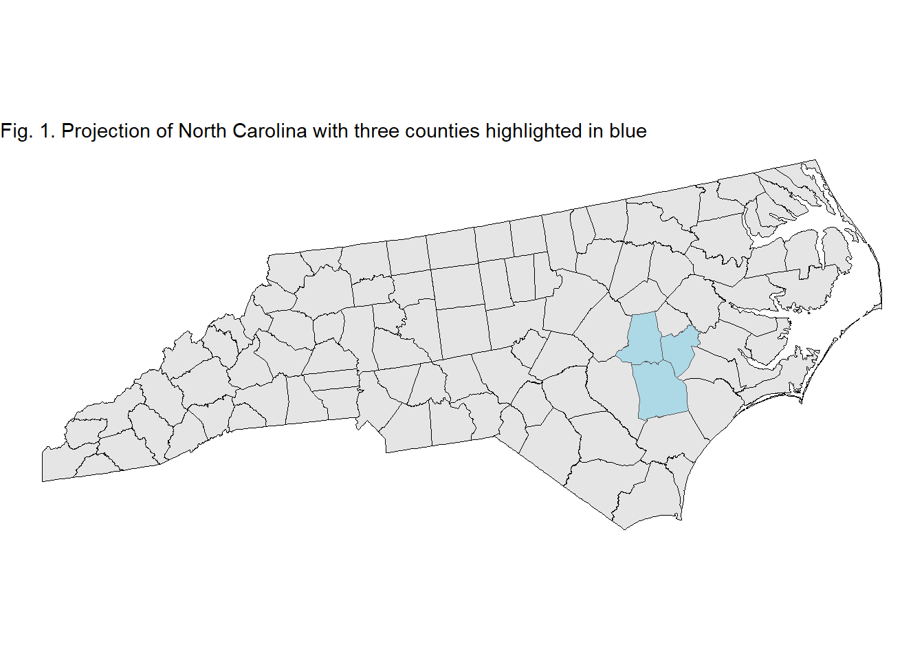
The code snippet creates a map of North Carolina using ggplot2 with the geom_sf() function to handle spatial data. The map highlights the entire state with a thin black outline, while three specific counties—Lenoir, Duplin, and Wayne—are filled with light blue to stand out.

Zonal raster data

To focus only on the fields within the selected counties, we can crop the raster and mask out non-agricultural area using raster::mask().

cdl_crop = crop(cdl, vect(NC_3))
csl_msk = rasterize(vect(NC_3), cdl_crop)
cdl_mbs = mask(cdl_crop, csl_msk)

Reclassifying crop types

We’ll reclassify the CDL into broader crop categories. The main crops in this region are corn (1), soybeans (5), and wheat (24, 26, 236, 238, 225), which we’ll combine into a single classes. We make all the other classes as 4. The crop coding can be found here.

oldclas = c(1, 5, 24, 26, 236, 238, 225)
newclas = c(1, 2, 3, 3, 3, 3, 3)
lookup = data.frame(oldclas, newclas)

cdl_rc = terra::classify(cdl_mbs, 
                         rcl = lookup, 
                         others = 4)

Visualizing corn, soybean, and wheat fields

Now we can visualize the reclassified raster with the county boundaries overlaid.

newnames = c("Corn", "Soybean","Wheat", "Other")
newcols <- c("yellow", 
             "green", 
             "tan", 
             "gray60")
newcols2 = colorspace::desaturate(newcols, amount = 0.2)

cdl_df = rasterdf(cdl_rc)

ggplot(data = cdl_df) +
  geom_raster(aes(x = x, y = y, fill = as.character(value))) + 
  scale_fill_manual(name = "Crop type",
                    values = newcols2,
                    labels = newnames,
                    na.translate = FALSE) +
  geom_sf(data = NC_3, fill = NA) +
  labs(subtitle = "Fig. 2. Cropland data layer in three counties in NC")+
  theme_void() +
  theme(strip.text.x = element_text(size=12, face="bold"))

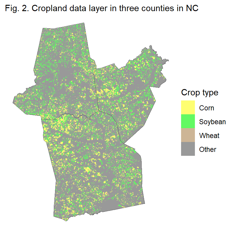
Everything looks good so far, but our goal is to sample coordinates across all wheat fields in North Carolina, not just in the selected counties. To achieve this, we’ll need to rerun some of the previous code, modifying it to work with the entire state.

Shifting Gears to State

Since the CDL file for the entire state is quite large, we’ll skip plotting it to avoid handling a heavy file.

cdl_crop = crop(cdl, vect(NC)) # NC instead of NC_3
## |---------|---------|---------|---------|=========================================                                          
csl_msk = rasterize(vect(NC), cdl_crop)
cdl_mbs = mask(cdl_crop, csl_msk)
## |---------|---------|---------|---------|=========================================                                          
oldclas = c(1, 5,24, 26, 236, 238, 225)
newclas = c(1, 2, 3, 3, 3, 3, 3)
lookup = data.frame(oldclas, newclas)

cdl_rc = terra::classify(cdl_mbs, 
                         rcl = lookup, 
                         others = 4)
## |---------|---------|---------|---------|=========================================                                          
wheat_fields = which(values(cdl_rc) == 3) # selecting wheat fields only
mask = cdl_rc
values(mask)[-wheat_fields] = NA

polygons_sf = st_as_sf(as.polygons(mask))
## |---------|---------|---------|---------|=========================================                                          

Randomly Sampling 100 Wheat Fields in North Carolina

Like it was done before for three counties, this code isolates wheat fields from the raster data and converts them into a polygonal vector format, making it easier to work with these areas in subsequent spatial analyses or sampling procedures.

Here, we sample 100 wheat fields in the entire state using the function st_sample.

set.seed(42) # Set seed for reproducibility
points = st_sample(polygons_sf, size =100)

ggplot() +
  geom_sf(data = NC, fill = NA) +
  geom_sf(data = points, fill = NA) +
  theme_void() +
  labs(subtitle = "Fig. 3. Geocoordinates of a hundred wheat fields in NC")+
  theme(strip.text.x = element_text(size=12, face="bold"))

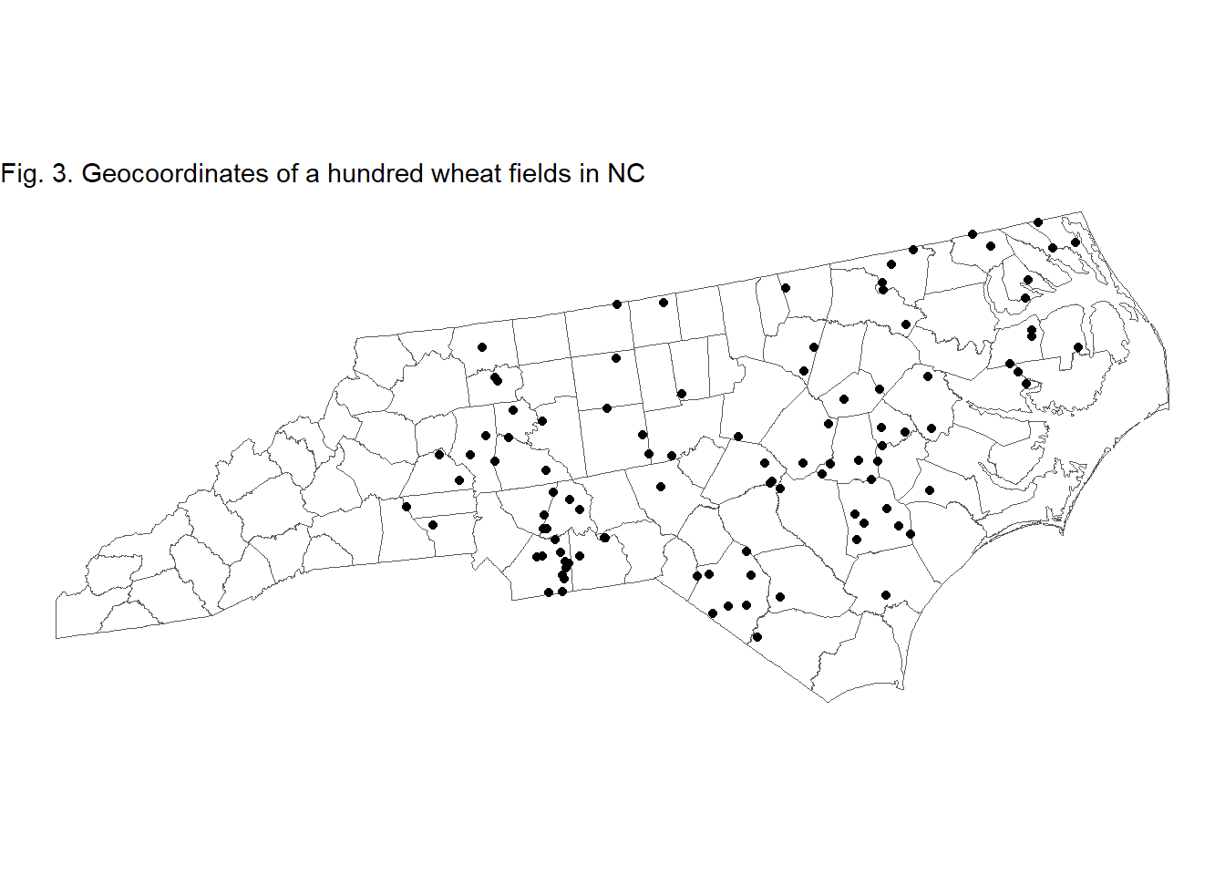
Create Geocoordinates

Finally, we’ll transform the points to geographic coordinates (longitude, latitude) and create a data frame with the results.

points = st_transform(points, crs = 4326)
coords_df = as.data.frame(st_coordinates(points))
coords_df$field_ID = 1:nrow(coords_df)
names(coords_df) = c("Lon", "Lat", "field_ID")

head(coords_df)
##         Lon      Lat field_ID
## 1 -80.64812 36.21178        1
## 2 -79.38605 35.54028        2
## 3 -76.44583 35.88619        3
## 4 -79.81857 35.90343        4
## 5 -79.56313 35.57671        5
## 6 -75.96710 36.36438        6

This completes the process of mapping and sampling wheat fields in North Carolina. The coordinates can now be used for metereological data download or fieldwork planning. The same workflow can be applied at another or for different crops by adjusting the parameters accordingly.

Vinicius Garnica
Vinicius Garnica
Research and Teaching Assistant

My research interests include agronomy and plant pathology matter.