Analysis of quantitative factors in split-plot design
Analysis of Messy Data Vol.2, Milliken and Johnson, 2009. pg 440
In this experiment, researchers are interested in evaluating the effect of moisture and fertilizer on dry weight of wheat. There were 48 different peat pots and 12 plastic trays; four pots could be put into each tray. The moisture treatments consisted of adding 10, 20, 30, or 40 ml of water per pot per day to the tray where the water was absorbed by the peat pots. The levels of moisture were randomly assigned to the trays. The trays are the large size of experimental unit or whole plot, and the whole plot design is a one-way treatment structure in a completely randomized design structure.
The levels of fertilizer were 2, 4, 6, or 8 mg per pot. The four levels of fertilizer were randomly assigned to the four pots in each tray so that each fertilizer occurred once in each tray. The pot is the smallest size of experimental unit or split-plot or subplot, and the subplot design is a one-way treatment structure in a randomized complete block design structure where the 12 trays are the blocks.
Loading packages
library(pacman)

p_load(lmerTest,
       reshape2,
       emmeans,
       plotly)

options(digits = 5,contrasts=c("contr.sum","contr.poly"))
NOTE: There may be better/easier ways to perform the analysis/data wrangling. Modifications are encouraged.
First, we need to transform the data from wide to long format. That can be done with melt function, as shown below. After reshaping the dataset and renaming variables, we create quantitative and qualitative variables, so we can perform ANOVA and estimate the regression coefficients.
Loading data
load("d:/R programs/Split-plot quantitative factors/data.RData")
data$Tray=as.factor(data$Tray)
data<- data %>% melt(id=c("MST","Tray"))
names(data)[3:4]<-c("FERT","Y")
data$fert= as.numeric(data$FERT)*2
data$mst= data$MST
data$MST1=as.factor(data$MST)
str(data)
## 'data.frame': 48 obs. of 7 variables:
## $ MST : int 10 10 10 20 20 20 30 30 30 40 ...
## $ Tray: Factor w/ 3 levels "1","2","3": 1 2 3 1 2 3 1 2 3 1 ...
## $ FERT: Factor w/ 4 levels "Fert2","Fert4",..: 1 1 1 1 1 1 1 1 1 1 ...
## $ Y : num 3.35 4.04 1.98 5.05 5.91 ...
## $ fert: num 2 2 2 2 2 2 2 2 2 2 ...
## $ mst : int 10 10 10 20 20 20 30 30 30 40 ...
## $ MST1: Factor w/ 4 levels "10","20","30",..: 1 1 1 2 2 2 3 3 3 4 ...Note that uppercase are factors and lowecase are numeric. Now we run anova using linear mixed model with lmer function from lme4 and lmerTest package.
Performing ANOVA in qualitative factors
lmer1<-lmer(Y~MST1*FERT+(1|Tray:MST),REML=TRUE,data=data)
anova(lmer1,ddf="Kenward-Roger")
## Type III Analysis of Variance Table with Kenward-Roger's method
## Sum Sq Mean Sq NumDF DenDF F value Pr(>F)
## MST1 59.4 19.8 3 8 26.34 0.00017 ***
## FERT 297.1 99.0 3 24 131.65 4.9e-15 ***
## MST1:FERT 38.1 4.2 9 24 5.62 0.00034 ***
## ---
## Signif. codes: 0 '***' 0.001 '**' 0.01 '*' 0.05 '.' 0.1 ' ' 1Main factors and interaction are statistically significant (P<0.05).
Visualizing the interaction
par(mfrow=c(1,2))
interaction.plot(data$MST1,data$FERT,data$Y)
interaction.plot(data$FERT,data$MST1,data$Y)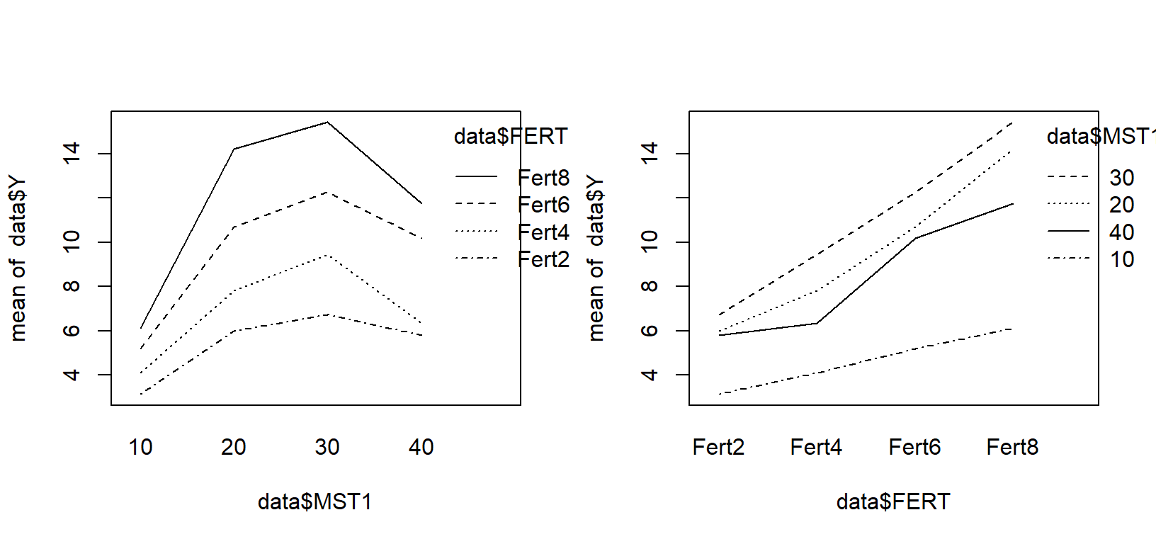
The graphs show the response to fertilizer for each moisture level and the response to moisture for each fertilizer level. It seems responses are quadratic for moisture and linear for fertilizer. We need to test that.
Variance components
print(VarCorr(lmer1),comp=c("Variance"),digits=4)## Groups Name Variance
## Tray:MST (Intercept) 0.6636
## Residual 0.7521Estimating the errors to test defined contrasts for linear, quadratic or cubic trends.
Contrasts
Fertilizer
There are four levels of fertilizer so the variance contrast to test linear trend at the same whole plot treatment (moisture) is:
\(\frac{\sigma^2_p}{3}[(-3)^2+(-1)^2+1^2+3^2] = \frac{20\sigma^2_p}{3}\)
and for quadratic trend is:
\[\frac{\sigma^2_p}{3}[(-1)^2+(-1)^2+1^2+1^2] = \frac{4\sigma^2_p}{3}\] and the cubic trend is:
\[\frac{\sigma^2_p}{3}[(-1)^2+(3)^2+(-3)^2+1^2] = \frac{20\sigma^2_p}{3}\]
The estimated standard errors are obtained by replacing \(\sigma^2\) with MSError(pot) in the square root of the respective variance (MSE=0.7521).
Moisture
Similarly, to test moisture (comparisons of whole plot treatments at the same subplot treatment) are: \[\frac{\sigma^2_{pot}+\sigma^2_{tray}}{3}[(-3)^2+(-1)^2+1^2+3^2] = \frac{20(\sigma^2_{pot}+\sigma^2_{tray})}{3}\] \[\frac{\sigma^2_{pot}+\sigma^2_{tray}}{3}[(-1)^2+(-1)^2+1^2+1^2] = \frac{4(\sigma^2_{pot}+\sigma^2_{tray})}{3}\] \[\frac{\sigma^2_{pot}+\sigma^2_{tray}}{3}[(-1)^2+(3)^2+(-3)^2+1^2] = \frac{20(\sigma^2_{pot}+\sigma^2_{tray})}{3}\]
for linear and quadratic, respectively. Variance components are inserted in the formula to obtain estimates of standard errors.
###Testing for significance of linear-quadratic-cubic trends.
emm1<-emmeans(lmer1,pairwise ~FERT|MST1)
contrast(emm1[[1]],"poly")
## MST1 = 10:
## contrast estimate SE df t.ratio p.value
## linear 10.0922 2.24 24 4.507 0.0001
## quadratic -0.0348 1.00 24 -0.035 0.9725
## cubic -0.2465 2.24 24 -0.110 0.9133
##
## MST1 = 20:
## contrast estimate SE df t.ratio p.value
## linear 27.6660 2.24 24 12.355 <.0001
## quadratic 1.6810 1.00 24 1.679 0.1062
## cubic -0.3504 2.24 24 -0.156 0.8770
##
## MST1 = 30:
## contrast estimate SE df t.ratio p.value
## linear 29.0017 2.24 24 12.951 <.0001
## quadratic 0.4346 1.00 24 0.434 0.6682
## cubic 0.1908 2.24 24 0.085 0.9328
##
## MST1 = 40:
## contrast estimate SE df t.ratio p.value
## linear 21.7646 2.24 24 9.720 <.0001
## quadratic 1.0478 1.00 24 1.046 0.3058
## cubic -5.5881 2.24 24 -2.495 0.0198
##
## Degrees-of-freedom method: kenward-rogerThere is a significant linear response to fertilizer for each level of moisture and no significant quadratic trend.
The Satterthwaite method can be used to approximate degrees of freedom associated with \(\sigma^2_{pot}+\sigma^2_{tray}\). As seen below, df=19.29.
emm2<-emmeans(lmer1,pairwise ~MST1|FERT)
contrast(emm2[[1]],"poly")
## FERT = Fert2:
## contrast estimate SE df t.ratio p.value
## linear 8.765 3.07 19.3 2.853 0.0101
## quadratic -3.768 1.37 19.3 -2.743 0.0128
## cubic 0.442 3.07 19.3 0.144 0.8872
##
## FERT = Fert4:
## contrast estimate SE df t.ratio p.value
## linear 8.303 3.07 19.3 2.703 0.0140
## quadratic -6.833 1.37 19.3 -4.973 0.0001
## cubic -2.596 3.07 19.3 -0.845 0.4085
##
## FERT = Fert6:
## contrast estimate SE df t.ratio p.value
## linear 16.583 3.07 19.3 5.398 <.0001
## quadratic -7.612 1.37 19.3 -5.540 <.0001
## cubic 0.261 3.07 19.3 0.085 0.9333
##
## FERT = Fert8:
## contrast estimate SE df t.ratio p.value
## linear 18.123 3.07 19.3 5.899 <.0001
## quadratic -11.779 1.37 19.3 -8.573 <.0001
## cubic 2.045 3.07 19.3 0.666 0.5136
##
## Degrees-of-freedom method: kenward-roger#Note that in the book, the estimates for the linear contrasts on level of moisture are incorrect...There are both linear and quadratic responses to moisture for each level of fertilizer.
Regression with split-plot errors
To obtain an appropriate analysis, one needs to use moisture as a continuous variable in the regression model and as a class variable in the random statement. “mst” is used to denote moisture as a continuous variable and “MST”” is used to denote the class variable. The random statement inserts the tray error term and imposes the correlation structure on the data.
Full model Y= \(\beta\)0 + \(\beta_1~_{mst}\) + \(\beta_2~_{mst{^2}}\) + \(\beta_3~_{mst{^3}}\) + \(\beta_4~_{fert}\) + \(\beta_5~_{fert{^2}}\) + \(\beta_6~_{fert{^3}}\) + \(\beta_7~_{mst*fert}\) + \(\beta_8~_{mst{^2}*fert}\) + \(\beta_9~_{mst{^3}*fert}\) + \(\beta_{10}~_{mst*fert{^2}}\) + \(\beta_{11}~_{fert{^2}*mst{^2}}\) + \(\beta_{12}~_{fert{^2}*mst{^3}}\) + \(\beta_{13}~_{mst*fert{^3}}\) + \(\beta_{14}~_{mst{^2}*fert{^3}}\) + \(\beta_{15} ~_{fert{^3}*mst{^3}}\) + tray(MST) + e.
lmer2a<-lmer(Y~mst+I(mst*mst)+I(mst*MST*MST)+fert+I(fert*fert)+I(fert*fert*fert)+I(mst*fert)+
              I(mst*mst*fert)+I(mst*mst*mst*fert)+I(mst*fert*fert)+I(mst*mst*fert*fert)+
              I(mst*mst*mst*fert*fert)+I(mst*fert*fert*fert)+I(mst*mst*fert*fert*fert)+I(mst*mst*mst*fert*fert*fert)+
              (1|MST1:Tray), REML = TRUE,data=data)

summary(lmer2a)
## Linear mixed model fit by REML. t-tests use Satterthwaite's method [
## lmerModLmerTest]
## Formula: Y ~ mst + I(mst * mst) + I(mst * MST * MST) + fert + I(fert *
## fert) + I(fert * fert * fert) + I(mst * fert) + I(mst * mst *
## fert) + I(mst * mst * mst * fert) + I(mst * fert * fert) +
## I(mst * mst * fert * fert) + I(mst * mst * mst * fert * fert) +
## I(mst * fert * fert * fert) + I(mst * mst * fert * fert *
## fert) + I(mst * mst * mst * fert * fert * fert) + (1 | MST1:Tray)
## Data: data
##
## REML criterion at convergence: 294.9
##
## Scaled residuals:
## Min 1Q Median 3Q Max
## -1.4208 -0.5731 -0.0921 0.4582 2.1132
##
## Random effects:
## Groups Name Variance Std.Dev.
## MST1:Tray (Intercept) 0.664 0.815
## Residual 0.752 0.867
## Number of obs: 48, groups: MST1:Tray, 12
##
## Fixed effects:
## Estimate Std. Error df t value
## (Intercept) -2.14e+01 3.48e+01 2.49e+01 -0.61
## mst 3.97e+00 5.32e+00 2.49e+01 0.75
## I(mst * mst) -1.86e-01 2.35e-01 2.49e+01 -0.79
## I(mst * MST * MST) 2.72e-03 3.12e-03 2.49e+01 0.87
## fert 1.48e+01 2.64e+01 2.41e+01 0.56
## I(fert * fert) -2.93e+00 5.84e+00 2.41e+01 -0.50
## I(fert * fert * fert) 1.56e-01 3.88e-01 2.41e+01 0.40
## I(mst * fert) -2.58e+00 4.04e+00 2.41e+01 -0.64
## I(mst * mst * fert) 1.33e-01 1.79e-01 2.41e+01 0.74
## I(mst * mst * mst * fert) -2.05e-03 2.37e-03 2.41e+01 -0.87
## I(mst * fert * fert) 5.26e-01 8.93e-01 2.41e+01 0.59
## I(mst * mst * fert * fert) -2.67e-02 3.94e-02 2.41e+01 -0.68
## I(mst * mst * mst * fert * fert) 4.13e-04 5.24e-04 2.41e+01 0.79
## I(mst * fert * fert * fert) -2.88e-02 5.93e-02 2.41e+01 -0.49
## I(mst * mst * fert * fert * fert) 1.52e-03 2.62e-03 2.41e+01 0.58
## I(mst * mst * mst * fert * fert * fert) -2.42e-05 3.48e-05 2.41e+01 -0.70
## Pr(>|t|)
## (Intercept) 0.54
## mst 0.46
## I(mst * mst) 0.44
## I(mst * MST * MST) 0.39
## fert 0.58
## I(fert * fert) 0.62
## I(fert * fert * fert) 0.69
## I(mst * fert) 0.53
## I(mst * mst * fert) 0.46
## I(mst * mst * mst * fert) 0.39
## I(mst * fert * fert) 0.56
## I(mst * mst * fert * fert) 0.50
## I(mst * mst * mst * fert * fert) 0.44
## I(mst * fert * fert * fert) 0.63
## I(mst * mst * fert * fert * fert) 0.57
## I(mst * mst * mst * fert * fert * fert) 0.49
## fit warnings:
## Some predictor variables are on very different scales: consider rescalingMost of the significance levels are quite large, so several steps of a deletion process were carried out until all of the remaining variables had coefficients that were significantly different from zero.
Reduced model Y= \(\beta\)0 + \(\beta_1~_{mst}\) + \(\beta_4~_{fert}\) + \(\beta_7~_{mst*fert}\) + \(\beta_8~_{mst{^2}*fert}\) + \(\beta_{10}~_{mst*fert{^2}}\) + tray(MST) + e.
It is of interest to determine if the reduced model adequately describes the data, so a lack of fit test is constructed.
Testing for lack of fit
lmer3<-lmer(Y~mst + fert + I(mst*fert) + I(mst*mst*fert)+ I(mst*fert*fert)+FERT:MST1+(1|Tray:MST1), REML = TRUE,data=data)
anova(lmer3,ddf="Kenward-Roger")
## Type III Analysis of Variance Table with Kenward-Roger's method
## Sum Sq Mean Sq NumDF DenDF F value Pr(>F)
## mst 0.06 0.06 1 27.3 0.08 0.7854
## fert 0.02 0.02 1 30.1 0.03 0.8616
## I(mst * fert) 7.92 7.92 1 18.1 10.53 0.0045 **
## I(mst * mst * fert) 6.29 6.29 1 19.3 8.37 0.0092 **
## I(mst * fert * fert) 2.58 2.58 1 24.0 3.43 0.0765 .
## FERT:MST1 6.83 0.68 10 24.7 0.89 0.5561
## ---
## Signif. codes: 0 '***' 0.001 '**' 0.01 '*' 0.05 '.' 0.1 ' ' 1The significance level corresponding to the test of lack of fi t is 0.5561, indicating the reduced model adequately describes the data.
Model Coefficients
lmer3a<-lmer(Y~mst + fert + I(mst*fert) + I(mst*mst*fert)+ I(mst*fert*fert)+(1|Tray:MST1), REML = TRUE,data=data)
summary(lmer3a)
## Linear mixed model fit by REML. t-tests use Satterthwaite's method [
## lmerModLmerTest]
## Formula: Y ~ mst + fert + I(mst * fert) + I(mst * mst * fert) + I(mst *
## fert * fert) + (1 | Tray:MST1)
## Data: data
##
## REML criterion at convergence: 178.4
##
## Scaled residuals:
## Min 1Q Median 3Q Max
## -2.5070 -0.5291 0.0653 0.4456 1.6692
##
## Random effects:
## Groups Name Variance Std.Dev.
## Tray:MST1 (Intercept) 0.558 0.747
## Residual 0.757 0.870
## Number of obs: 48, groups: Tray:MST1, 12
##
## Fixed effects:
## Estimate Std. Error df t value Pr(>|t|)
## (Intercept) 1.953558 0.920448 32.987398 2.12 0.041 *
## mst 0.075312 0.040690 40.622841 1.85 0.071 .
## fert -1.079512 0.231841 37.847605 -4.66 3.9e-05 ***
## I(mst * fert) 0.172963 0.022470 36.511857 7.70 3.7e-09 ***
## I(mst * mst * fert) -0.003463 0.000373 25.441178 -9.28 1.2e-09 ***
## I(mst * fert * fert) 0.001838 0.001147 32.437572 1.60 0.119
## ---
## Signif. codes: 0 '***' 0.001 '**' 0.01 '*' 0.05 '.' 0.1 ' ' 1
##
## Correlation of Fixed Effects:
## (Intr) mst fert I(*fr) I(*m*f
## mst -0.754
## fert -0.444 0.335
## I(mst*fert) 0.153 -0.426 -0.789
## I(ms*m*frt) 0.000 0.000 0.805 -0.830
## I(ms*f*frt) 0.000 0.564 0.000 -0.510 0.000
## fit warnings:
## Some predictor variables are on very different scales: consider rescalingTransforming the factors back to numeric.
a<-data.frame(emmeans(lmer1,~FERT*MST1))[,1:3]
a$FERT=as.numeric(a$FERT)*2
a$MST1=as.numeric(a$MST1)*10
Using the model to predict surface with an expanded dataset.
pred_grid <- expand.grid(fert= seq(2,8, by=0.5), mst  = seq(10,40, by=1))
predicted=function(x,y){
  z=1.9535+x*0.07531-y*1.07951+x*y*0.17296-x*x*y*0.003463+x*y*y*0.0018379
}
pred_grid$predicted<-predicted(pred_grid$mst,pred_grid$fert)

plot_ly(x = ~pred_grid$mst, y = ~pred_grid$fert, z = ~pred_grid$predicted, type = "mesh3d") %>%
  add_markers(x = ~a$MST1, y = ~a$FERT, z = ~a$emmean) %>%
  layout(scene = list(xaxis = list(title = 'Moisture'),
                     yaxis = list(title = 'Fertilizer'),
                     zaxis = list(title = 'Dry matter mean')))
The surface was fit with the reduced model indicated above. The regression model does a good job of describing the cell means (orange circles).
Vini Garnica
Assistant Professor
Quantitative plant pathologist developing data-driven tools for disease prediction and crop management.